Below is code determining the samples with possible chr11 fragment duplication and breaking down the counts of perfect duplicated copies vs divergent copies.
Calculating the population of the haplotypes after the shared region on chr 11, the duplicated region to see if there is any population signal associated with the duplicated copy. E.g. if the copy is unique to a subset of haplotypes, if the copy is always perfect or if there is variation.
Samples with a duplicated chromosome 11 and deleted chr 13 (Pattern 1 of HRP3 deletion)
Jacard index of the duplicated region on chromosome 11, jacard of 1 means complete agreement between samples on this region which 0 would be no haplotypes shared in this region. Additional meta data of the samples is shown on top and to the right including country/region, and the hrp2/3 calls, whether the the Chr11 that has been duplicated is a perfect copy or not.
It appears the African samples and South American samples, while related within continent, are not very closely related to each other.
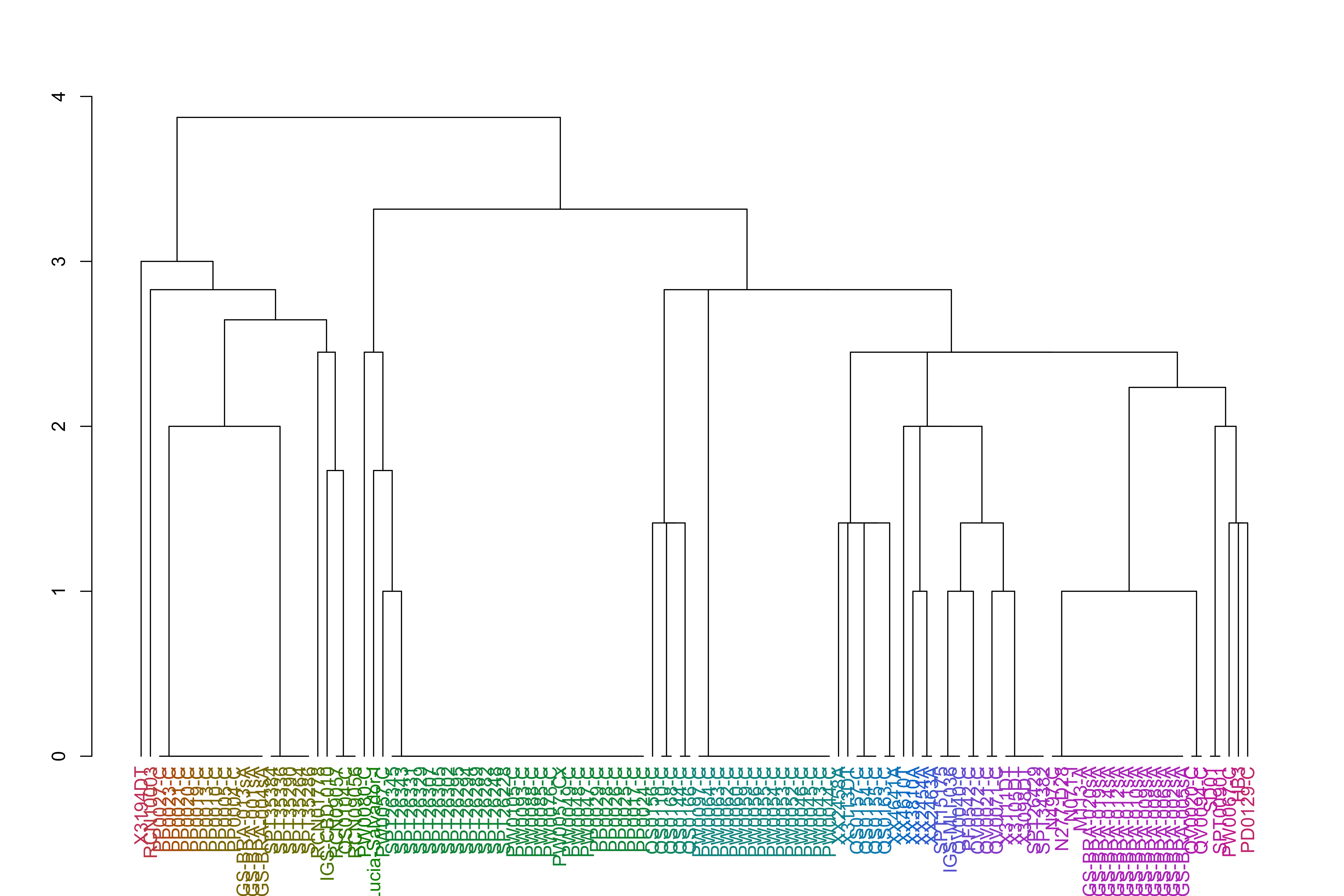
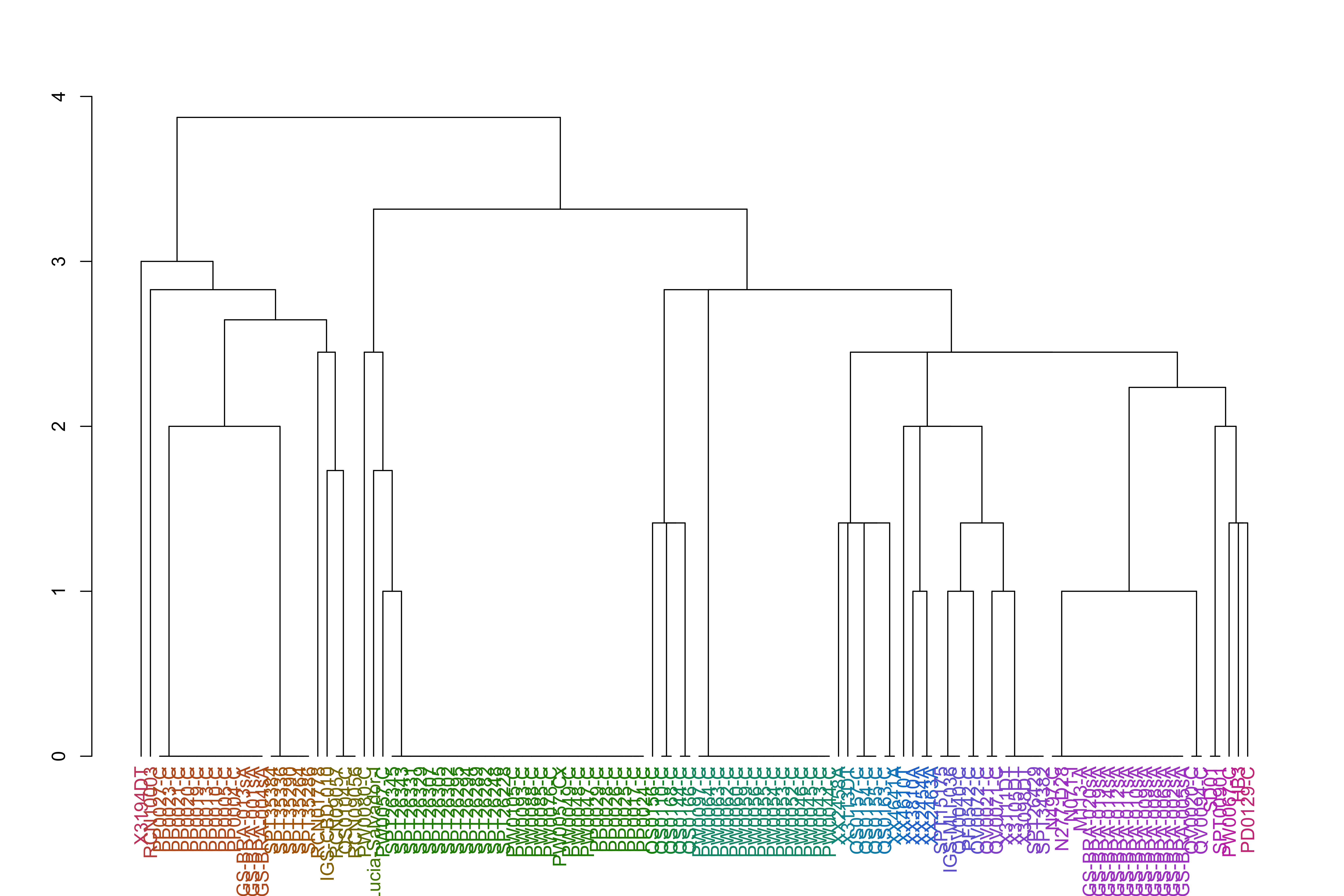
Plotting out the variation at the duplicated region, coloring haplotypes by their abundance rank, this visualization will allow interpretation of how similar these haplotypes are here and what the copy looks like within sample (e.g. perfect copy vs variation and how much variation )
All samples with pattern 1 HRP3 deletion
Code
varCounts_filt_hrp3_pat1_regions_afterHomologous_chr11_prep=HaplotypeRainbows::prepForRainbow(varCounts_filt_hrp3_pat1_regions_afterHomologous_chr11, minPopSize =1)# select just the major haplotypes and cluster based on the sharing betweenvarCounts_filt_hrp3_pat1_regions_afterHomologous_chr11_prep_sp=varCounts_filt_hrp3_pat1_regions_afterHomologous_chr11_prep%>%group_by(p_name)%>%mutate(sampleCount =length(unique(s_Sample)))%>%group_by()%>%filter(sampleCount>=0.99*max(sampleCount))%>%group_by(s_Sample, p_name)%>%#filter(c_AveragedFrac == max(c_AveragedFrac)) %>% mutate(marker =1)%>%group_by()%>%select(h_popUID, marker, s_Sample)%>%spread(h_popUID, marker, fill =0)varCounts_filt_hrp3_pat1_regions_afterHomologous_chr11_prep_sp_mat=as.matrix(varCounts_filt_hrp3_pat1_regions_afterHomologous_chr11_prep_sp[,2:ncol(varCounts_filt_hrp3_pat1_regions_afterHomologous_chr11_prep_sp)])rownames(varCounts_filt_hrp3_pat1_regions_afterHomologous_chr11_prep_sp_mat)=varCounts_filt_hrp3_pat1_regions_afterHomologous_chr11_prep_sp$s_SamplevarCounts_filt_hrp3_pat1_regions_afterHomologous_chr11_prep_sp_dist=dist(varCounts_filt_hrp3_pat1_regions_afterHomologous_chr11_prep_sp_mat)varCounts_filt_hrp3_pat1_regions_afterHomologous_chr11_prep_sp_dist_hclust=hclust(varCounts_filt_hrp3_pat1_regions_afterHomologous_chr11_prep_sp_dist)jacardDist_gat_filt_sp_mat_pat1_hc=hclust(dist(jacardDist_gat_filt_sp_mat_pat1))#rename the levels so they are in the order of the clustering varCounts_filt_hrp3_pat1_regions_afterHomologous_chr11_prep=varCounts_filt_hrp3_pat1_regions_afterHomologous_chr11_prep%>%mutate(s_Sample =factor(s_Sample, levels =rownames(varCounts_filt_hrp3_pat1_regions_afterHomologous_chr11_prep_sp_mat)[varCounts_filt_hrp3_pat1_regions_afterHomologous_chr11_prep_sp_dist_hclust$order]))%>%# levels = rownames(jacardDist_gat_filt_sp_mat_pat1)[jacardDist_gat_filt_sp_mat_pat1_hc$order])) %>%mutate(popid =ifelse(maxPopid==1, -1, popid))varCounts_filt_hrp3_pat1_regions_afterHomologous_chr11_prep_plot=genRainbowHapPlotObj(varCounts_filt_hrp3_pat1_regions_afterHomologous_chr11_prep, colorCol =popid)+theme(axis.text.x =element_text(size=12, angle =-90, vjust =0.5, hjust =0))+scale_x_continuous(breaks =1:length(levels(varCounts_filt_hrp3_pat1_regions_afterHomologous_chr11_prep$p_name)), labels =levels(varCounts_filt_hrp3_pat1_regions_afterHomologous_chr11_prep$p_name), expand =c(0,0))+scale_y_continuous(expand =c(0,0))meta_varCounts_filt_hrp3_pat1_regions_afterHomologous_chr11_prep=meta_preferredSample%>%filter(BiologicalSample%in%varCounts_filt_hrp3_pat1_regions_afterHomologous_chr11_prep$s_Sample)%>%mutate(BiologicalSample =factor(BiologicalSample, levels =levels(varCounts_filt_hrp3_pat1_regions_afterHomologous_chr11_prep$s_Sample)))allColors=c(); for(nameinnames(rowAnnoColors)){allColors=c(allColors, rowAnnoColors[[name]])}previousColors=unique(ggplot_build(varCounts_filt_hrp3_pat1_regions_afterHomologous_chr11_prep_plot)$data[[1]][["fill"]])names(previousColors)=sort(unique(varCounts_filt_hrp3_pat1_regions_afterHomologous_chr11_prep$popid))previousColors["-1"]="grey0";allColors=c(allColors, previousColors)varCounts_filt_hrp3_pat1_regions_afterHomologous_chr11_prep_withCountry=varCounts_filt_hrp3_pat1_regions_afterHomologous_chr11_prep%>%mutate(s_Sample =factor(s_Sample, levels =rownames(varCounts_filt_hrp3_pat1_regions_afterHomologous_chr11_prep_sp_mat)[varCounts_filt_hrp3_pat1_regions_afterHomologous_chr11_prep_sp_dist_hclust$order]))%>%mutate(popid=factor(popid))
Code
varCounts_filt_hrp3_pat1_regions_afterHomologous_chr11_prep_withCountry_plot_mod1=genRainbowHapPlotObj(varCounts_filt_hrp3_pat1_regions_afterHomologous_chr11_prep_withCountry, colorCol =popid)+theme(axis.text.x =element_text(size=12, angle =-90, vjust =0.5, hjust =0))+scale_x_continuous(breaks =c(-19.5+2.25, -14.5+2.25, -9.5+2.25, -4.5+2.25, 1:length(levels(varCounts_filt_hrp3_pat1_regions_afterHomologous_chr11_prep_withCountry$p_name))), labels =c("Chr11DupHapCluster", "continent", "region", "country",# levels(varCounts_filt_hrp3_pat1_regions_afterHomologous_chr11_prep_withCountry$p_name), rep("", length(levels(varCounts_filt_hrp3_pat1_regions_afterHomologous_chr11_prep_withCountry$p_name)))), expand =c(0,0))+scale_y_continuous( expand =c(0, 0), breaks =1:length(levels(varCounts_filt_hrp3_pat1_regions_afterHomologous_chr11_prep_withCountry$s_Sample)), labels =levels(varCounts_filt_hrp3_pat1_regions_afterHomologous_chr11_prep_withCountry$s_Sample))rowAnnoColors[["Chr11DupHapCluster"]]=popClustering_filt_hrp3_pat1_regions_afterHomologous_chr11_prep_forClustering_sp_dist_hclust_groups_df$colorsnames(rowAnnoColors[["Chr11DupHapCluster"]])=popClustering_filt_hrp3_pat1_regions_afterHomologous_chr11_prep_forClustering_sp_dist_hclust_groups_df$Chr11DupHapClustervarCounts_filt_hrp3_pat1_regions_afterHomologous_chr11_prep_withCountry_plot_mod1=varCounts_filt_hrp3_pat1_regions_afterHomologous_chr11_prep_withCountry_plot_mod1+scale_fill_manual("SNP\nRank", values =haplotypeRankColors[sort(names(previousColors))], labels =names(haplotypeRankColors[sort(names(previousColors))]), breaks =names(haplotypeRankColors[sort(names(previousColors))]))+guides(fill =guide_legend(nrow =3))+ggnewscale::new_scale_fill()+geom_rect(aes(xmin=0, xmax =-4.5, ymin =as.numeric(BiologicalSample)-0.5, ymax =as.numeric(BiologicalSample)+0.5, fill =country), color ="black", data =meta_varCounts_filt_hrp3_pat1_regions_afterHomologous_chr11_prep)+scale_fill_manual("country", values =rowAnnoColors[["country"]])+guides(fill =guide_legend(nrow =3))+ggnewscale::new_scale_fill()+geom_rect(aes(xmin=-5, xmax =-9.5, ymin =as.numeric(BiologicalSample)-0.5, ymax =as.numeric(BiologicalSample)+0.5, fill =region), color ="black", data =meta_varCounts_filt_hrp3_pat1_regions_afterHomologous_chr11_prep)+scale_fill_manual("region", values =rowAnnoColors[["region"]])+guides(fill =guide_legend(nrow =3))+ggnewscale::new_scale_fill()+geom_rect(aes(xmin=-10, xmax =-14.5, ymin =as.numeric(BiologicalSample)-0.5, ymax =as.numeric(BiologicalSample)+0.5, fill =secondaryRegion), color ="black", data =meta_varCounts_filt_hrp3_pat1_regions_afterHomologous_chr11_prep)+scale_fill_manual("Continent", values =rowAnnoColors[["continent"]])+guides(fill =guide_legend(nrow =3))+ggnewscale::new_scale_fill()+geom_rect(aes(xmin=-15, xmax =-19.5, ymin =as.numeric(BiologicalSample)-0.5, ymax =as.numeric(BiologicalSample)+0.5, fill =Chr11DupHapCluster), color ="black", data =meta_varCounts_filt_hrp3_pat1_regions_afterHomologous_chr11_prep)+scale_fill_manual("Chr11DupHapCluster", values =rowAnnoColors[["Chr11DupHapCluster"]])+guides(fill =guide_legend(nrow =3))
The y axis is samples and the x-axis is sub region within the chromosome, sorted by genomic position. Haplotypes are colored by their abundance rank and while colors in a vertical column are the same haplotype, the same colors between column do not mean same haplotype. Rank is ordered by frequency within the total population. Columns with black bars are columns where there is no haplotype variation. Bar heights are relative to abundance within sample, so a sample with just 1 bar for a genomic position means monoclonal at this position while multiple bars would indicated polyclonal (and in this instance would mean the copy on chr11 and chr13 is not a perfect copy).
Code
regions_afterHomologous_chr11_filt=regions_afterHomologous_chr11%>%filter(genomicID%in%varCounts_filt_hrp3_pat1_regions_afterHomologous_chr11_prep$p_name)%>%mutate(genomicID =factor(genomicID, levels =levels(varCounts_filt_hrp3_pat1_regions_afterHomologous_chr11_prep$p_name)))varCounts_filt_hrp3_pat1_regions_afterHomologous_chr11_prep_withCountry_plot_mod1=varCounts_filt_hrp3_pat1_regions_afterHomologous_chr11_prep_withCountry_plot_mod1+new_scale_fill()+geom_rect(aes(xmin =as.numeric(genomicID)-0.5, xmax =as.numeric(genomicID)+0.5, ymax =0, ymin =-5, fill =description), data =regions_afterHomologous_chr11_filt, color ="black")+scale_fill_manual("Genes\nDescription", values =descriptionColors, guide =guide_legend(nrow =5))+transparentBackground+theme(legend.text =element_text(size =30), legend.title =element_text(size =30, face ="bold"), legend.box="vertical", legend.margin=margin(), legend.background =element_blank(), legend.box.background =element_rect(colour ="black"), axis.text.x =element_text(size =30))print(varCounts_filt_hrp3_pat1_regions_afterHomologous_chr11_prep_withCountry_plot_mod1)
varCounts_filt_hrp3_pat1_regions_afterHomologous_chr11_prep_sp_dist_hclust_groups=cutree(varCounts_filt_hrp3_pat1_regions_afterHomologous_chr11_prep_sp_dist_hclust, h =h_groups)varCounts_filt_hrp3_pat1_regions_afterHomologous_chr11_prep_sp_dist_hclust_dend<-as.dendrogram(varCounts_filt_hrp3_pat1_regions_afterHomologous_chr11_prep_sp_dist_hclust)varCounts_filt_hrp3_pat1_regions_afterHomologous_chr11_prep_sp_dist_hclust_dend<-color_labels(varCounts_filt_hrp3_pat1_regions_afterHomologous_chr11_prep_sp_dist_hclust_dend, h =h_groups)plot(varCounts_filt_hrp3_pat1_regions_afterHomologous_chr11_prep_sp_dist_hclust_dend)
Code
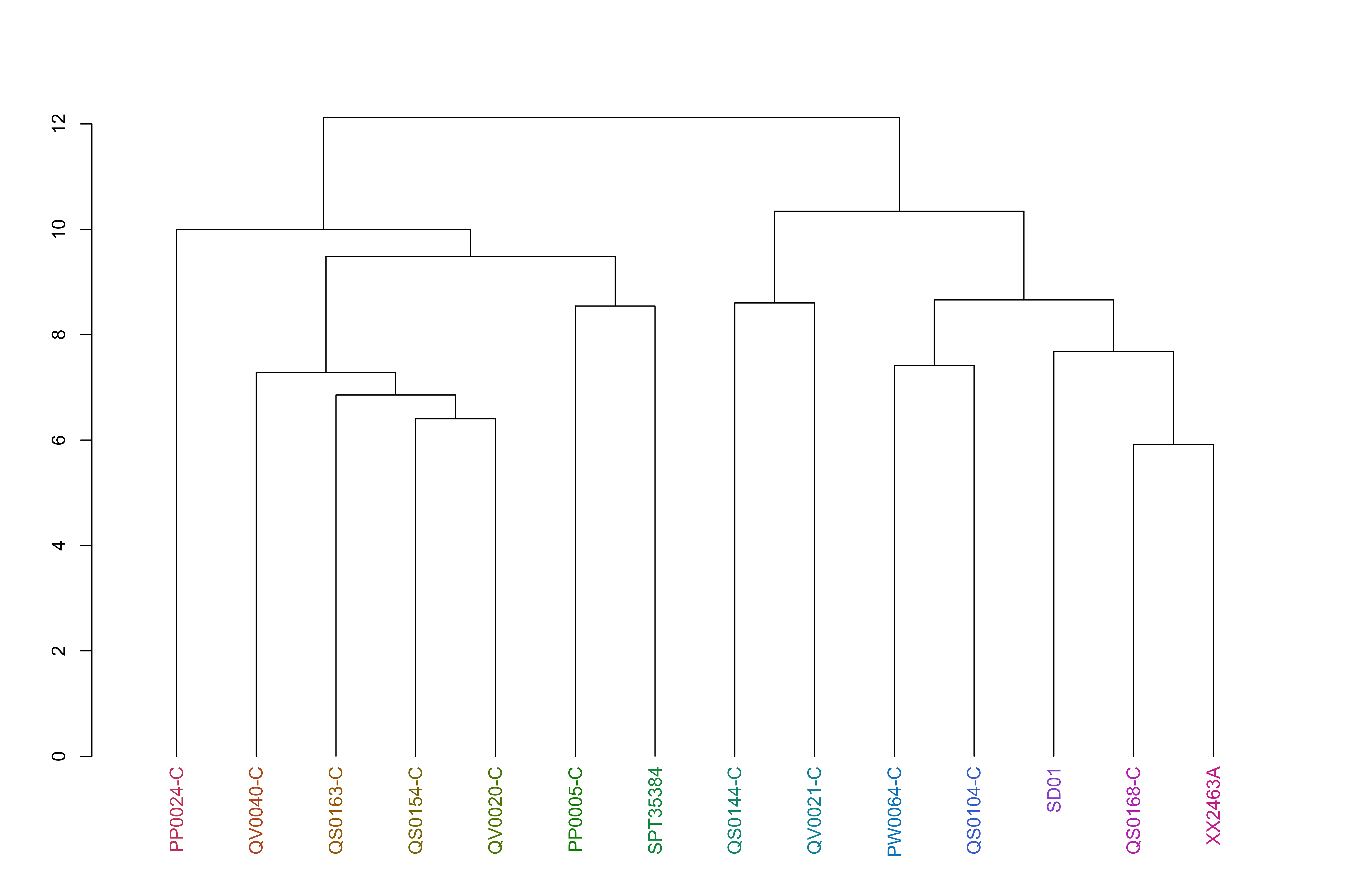
jacardDist_gat_filt_sp_mat_pat1_hc_groups=cutree(jacardDist_gat_filt_sp_mat_pat1_hc, k =k_groups)jacardDist_gat_filt_sp_mat_pat1_hc_dend<-as.dendrogram(jacardDist_gat_filt_sp_mat_pat1_hc)jacardDist_gat_filt_sp_mat_pat1_hc_dend<-color_labels(jacardDist_gat_filt_sp_mat_pat1_hc_dend, k =k_groups)plot(jacardDist_gat_filt_sp_mat_pat1_hc_dend)
Code
varCounts_filt_hrp3_pat1_regions_afterHomologous_chr11_prep_sp_dist_hclust_groups_df=tibble( BiologicalSample =names(varCounts_filt_hrp3_pat1_regions_afterHomologous_chr11_prep_sp_dist_hclust_groups), hcclust_variant =varCounts_filt_hrp3_pat1_regions_afterHomologous_chr11_prep_sp_dist_hclust_groups)%>%mutate(BiologicalSample =factor(BiologicalSample, levels =levels(meta_varCounts_filt_hrp3_pat1_regions_afterHomologous_chr11_prep$BiologicalSample)))jacardDist_gat_filt_sp_mat_pat1_hc_groups_df=tibble( BiologicalSample =names(jacardDist_gat_filt_sp_mat_pat1_hc_groups), hcclust_variant =jacardDist_gat_filt_sp_mat_pat1_hc_groups)%>%mutate(BiologicalSample =factor(BiologicalSample, levels =levels(meta_varCounts_filt_hrp3_pat1_regions_afterHomologous_chr11_prep$BiologicalSample)))varCounts_filt_hrp3_pat1_regions_afterHomologous_chr11_prep_withCountry_plot_mod2=varCounts_filt_hrp3_pat1_regions_afterHomologous_chr11_prep_withCountry_plot_mod2+scale_fill_manual("SNP\nRank", values =haplotypeRankColors[sort(names(previousColors))], labels =names(haplotypeRankColors[sort(names(previousColors))]), breaks =names(haplotypeRankColors[sort(names(previousColors))]))+guides(fill =guide_legend(nrow =5))+ggnewscale::new_scale_fill()+geom_rect(aes(xmin=0, xmax =-4.5, ymin =as.numeric(BiologicalSample)-0.5, ymax =as.numeric(BiologicalSample)+0.5, fill =secondaryRegion), color ="black", data =meta_varCounts_filt_hrp3_pat1_regions_afterHomologous_chr11_prep)+scale_fill_manual("Continent", values =rowAnnoColors[["continent"]])+guides(fill =guide_legend(nrow =4))+ggnewscale::new_scale_fill()+geom_rect(aes(xmin=-5, xmax =-9.5, ymin =as.numeric(BiologicalSample)-0.5, ymax =as.numeric(BiologicalSample)+0.5, fill =factor(hcclust_variant)), color ="black", data =varCounts_filt_hrp3_pat1_regions_afterHomologous_chr11_prep_sp_dist_hclust_groups_df)+# fill = factor(hcclust_variant)), color = "black", data = jacardDist_gat_filt_sp_mat_pat1_hc_groups_df)+ scale_fill_manual("HaploGroup", values =scheme$hex(length(unique(varCounts_filt_hrp3_pat1_regions_afterHomologous_chr11_prep_sp_dist_hclust_groups))))+guides(fill =guide_legend(nrow =5))regions_afterHomologous_chr11_filt=regions_afterHomologous_chr11%>%filter(genomicID%in%varCounts_filt_hrp3_pat1_regions_afterHomologous_chr11_prep$p_name)%>%mutate(genomicID =factor(genomicID, levels =levels(varCounts_filt_hrp3_pat1_regions_afterHomologous_chr11_prep$p_name)))yLabels_varCounts_filt_hrp3_pat1_regions_afterHomologous_chr11_prep_withCountry_plot_mod2=levels(varCounts_filt_hrp3_pat1_regions_afterHomologous_chr11_prep_withCountry$s_Sample)yLabels_varCounts_filt_hrp3_pat1_regions_afterHomologous_chr11_prep_withCountry_plot_mod2[yLabels_varCounts_filt_hrp3_pat1_regions_afterHomologous_chr11_prep_withCountry_plot_mod2%!in%c("HB3", "Santa-Lucia-Salvador-I", "SD01")]=""varCounts_filt_hrp3_pat1_regions_afterHomologous_chr11_prep_withCountry_plot_mod2=varCounts_filt_hrp3_pat1_regions_afterHomologous_chr11_prep_withCountry_plot_mod2+scale_y_continuous(labels =yLabels_varCounts_filt_hrp3_pat1_regions_afterHomologous_chr11_prep_withCountry_plot_mod2, breaks =1:length(yLabels_varCounts_filt_hrp3_pat1_regions_afterHomologous_chr11_prep_withCountry_plot_mod2), expand =c(0,0))+theme(axis.text.x =element_blank(), axis.line.x =element_blank(), axis.ticks.x =element_blank(), axis.title.x =element_blank(), axis.line.y =element_blank(), axis.ticks.y =element_blank(), axis.text.y =element_blank(), axis.title.y =element_blank(), panel.border =element_blank(), )varCounts_filt_hrp3_pat1_regions_afterHomologous_chr11_prep_withCountry_plot_mod2_priorToGeneInfo=varCounts_filt_hrp3_pat1_regions_afterHomologous_chr11_prep_withCountry_plot_mod2varCounts_filt_hrp3_pat1_regions_afterHomologous_chr11_prep_withCountry_plot_mod2=varCounts_filt_hrp3_pat1_regions_afterHomologous_chr11_prep_withCountry_plot_mod2+new_scale_fill()+geom_rect(aes(xmin =as.numeric(genomicID)-0.5, xmax =as.numeric(genomicID)+0.5, ymax =0, ymin =-7, fill =description), data =regions_afterHomologous_chr11_filt, color ="black")+geom_text(aes(y =as.numeric(BiologicalSample), x =-10, label =BiologicalSample), hjust =1, data =tibble(BiologicalSample =factor(c("HB3", "Santa-Lucia-Salvador-I", "SD01"), levels =levels(varCounts_filt_hrp3_pat1_regions_afterHomologous_chr11_prep_withCountry$s_Sample))))+scale_fill_manual("Genes\nDescription", values =descriptionColors, guide =guide_legend(nrow =5))
The y axis is samples and the x-axis is sub region within the chromosome, sorted by genomic position. Haplotypes are colored by their abundance rank and while colors in a vertical column are the same haplotype, the same colors between column do not mean same haplotype. Rank is ordered by frequency within the total population. Columns with black bars are columns where there is no haplotype variation. Bar heights are relative to abundance within sample, so a sample with just 1 bar for a genomic position means monoclonal at this position while multiple bars would indicated polyclonal (and in this instance would mean the copy on chr11 and chr13 is not a perfect copy).
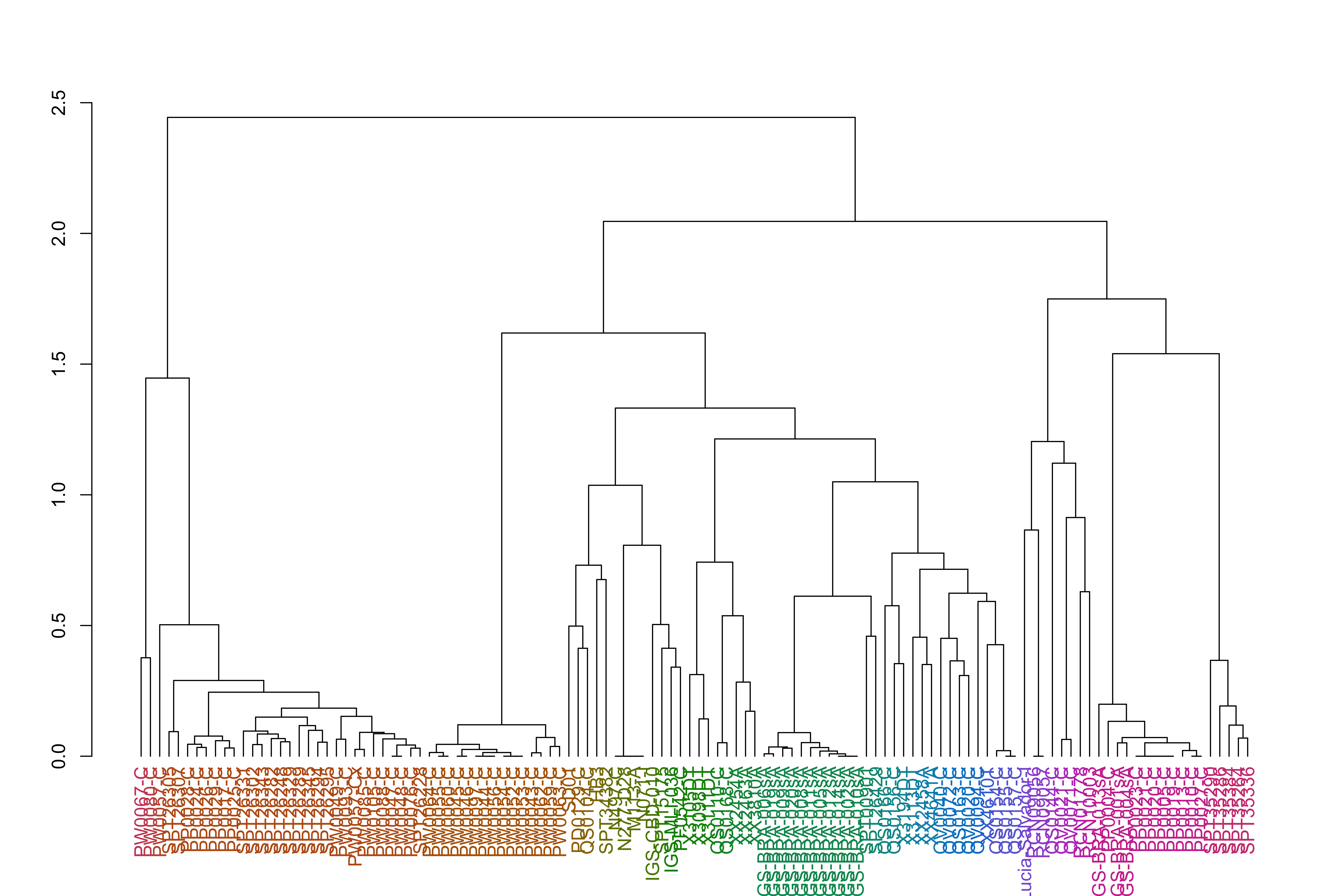
varCounts_filt_hrp3_pat1_regions_afterHomologous_chr11_prep_mod3=HaplotypeRainbows::prepForRainbow(varCounts_filt_hrp3_pat1_regions_afterHomologous_chr11, minPopSize =2)# select just the major haplotypes and cluster based on the sharing betweenvarCounts_filt_hrp3_pat1_regions_afterHomologous_chr11_prep_mod3_sp=varCounts_filt_hrp3_pat1_regions_afterHomologous_chr11_prep_mod3%>%group_by(p_name)%>%mutate(sampleCount =length(unique(s_Sample)))%>%group_by()%>%filter(sampleCount>=0.99*max(sampleCount))%>%group_by(s_Sample, p_name)%>%#filter(c_AveragedFrac == max(c_AveragedFrac)) %>% mutate(marker =1)%>%group_by()%>%select(h_popUID, marker, s_Sample)%>%spread(h_popUID, marker, fill =0)varCounts_filt_hrp3_pat1_regions_afterHomologous_chr11_prep_mod3_sp_mat=as.matrix(varCounts_filt_hrp3_pat1_regions_afterHomologous_chr11_prep_mod3_sp[,2:ncol(varCounts_filt_hrp3_pat1_regions_afterHomologous_chr11_prep_mod3_sp)])rownames(varCounts_filt_hrp3_pat1_regions_afterHomologous_chr11_prep_mod3_sp_mat)=varCounts_filt_hrp3_pat1_regions_afterHomologous_chr11_prep_mod3_sp$s_SamplevarCounts_filt_hrp3_pat1_regions_afterHomologous_chr11_prep_mod3_sp_dist=dist(varCounts_filt_hrp3_pat1_regions_afterHomologous_chr11_prep_mod3_sp_mat)varCounts_filt_hrp3_pat1_regions_afterHomologous_chr11_prep_mod3_sp_dist_hclust=hclust(varCounts_filt_hrp3_pat1_regions_afterHomologous_chr11_prep_mod3_sp_dist)jacardDist_gat_filt_sp_mat_pat1_hc=hclust(dist(jacardDist_gat_filt_sp_mat_pat1))#rename the levels so they are in the order of the clustering varCounts_filt_hrp3_pat1_regions_afterHomologous_chr11_prep_mod3=varCounts_filt_hrp3_pat1_regions_afterHomologous_chr11_prep_mod3%>%mutate(s_Sample =factor(s_Sample, levels =rownames(varCounts_filt_hrp3_pat1_regions_afterHomologous_chr11_prep_mod3_sp_mat)[varCounts_filt_hrp3_pat1_regions_afterHomologous_chr11_prep_mod3_sp_dist_hclust$order]))%>%# levels = rownames(jacardDist_gat_filt_sp_mat_pat1)[jacardDist_gat_filt_sp_mat_pat1_hc$order])) %>%mutate(popid =ifelse(maxPopid==1, -1, popid))varCounts_filt_hrp3_pat1_regions_afterHomologous_chr11_prep_mod3_plot=genRainbowHapPlotObj(varCounts_filt_hrp3_pat1_regions_afterHomologous_chr11_prep_mod3, colorCol =popid)+theme(axis.text.x =element_text(size=12, angle =-90, vjust =0.5, hjust =0))+scale_x_continuous(breaks =1:length(levels(varCounts_filt_hrp3_pat1_regions_afterHomologous_chr11_prep_mod3$p_name)), labels =levels(varCounts_filt_hrp3_pat1_regions_afterHomologous_chr11_prep_mod3$p_name), expand =c(0,0))meta_varCounts_filt_hrp3_pat1_regions_afterHomologous_chr11_prep_mod3=meta_preferredSample%>%filter(BiologicalSample%in%varCounts_filt_hrp3_pat1_regions_afterHomologous_chr11_prep_mod3$s_Sample)%>%mutate(BiologicalSample =factor(BiologicalSample, levels =levels(varCounts_filt_hrp3_pat1_regions_afterHomologous_chr11_prep_mod3$s_Sample)))allColors=c(); for(nameinnames(rowAnnoColors)){allColors=c(allColors, rowAnnoColors[[name]])}previousColors=unique(ggplot_build(varCounts_filt_hrp3_pat1_regions_afterHomologous_chr11_prep_mod3_plot)$data[[1]][["fill"]])names(previousColors)=sort(unique(varCounts_filt_hrp3_pat1_regions_afterHomologous_chr11_prep_mod3$popid))previousColors["-1"]="grey0";allColors=c(allColors, previousColors)varCounts_filt_hrp3_pat1_regions_afterHomologous_chr11_prep_mod3_withCountry=varCounts_filt_hrp3_pat1_regions_afterHomologous_chr11_prep_mod3%>%mutate(s_Sample =factor(s_Sample, levels =rownames(varCounts_filt_hrp3_pat1_regions_afterHomologous_chr11_prep_mod3_sp_mat)[varCounts_filt_hrp3_pat1_regions_afterHomologous_chr11_prep_mod3_sp_dist_hclust$order]))%>%mutate(popid=factor(popid))varCounts_filt_hrp3_pat1_regions_afterHomologous_chr11_prep_withCountry_plot_mod3=genRainbowHapPlotObj(varCounts_filt_hrp3_pat1_regions_afterHomologous_chr11_prep_mod3_withCountry, colorCol =popid)+theme(axis.text.x =element_text(size=12, angle =-90, vjust =0.5, hjust =0))+scale_x_continuous(limits =c(-30, max(c(-9.5+2.25, -4.5+2.25, 1:length(levels(varCounts_filt_hrp3_pat1_regions_afterHomologous_chr11_prep_mod3_withCountry$p_name))))), breaks =c(-9.5+2.25, -4.5+2.25, 1:length(levels(varCounts_filt_hrp3_pat1_regions_afterHomologous_chr11_prep_mod3_withCountry$p_name))), labels =c("HaploGroup", "continent", levels(varCounts_filt_hrp3_pat1_regions_afterHomologous_chr11_prep_mod3_withCountry$p_name)), expand =c(0,0))# k_groups = 20;# h_groups = 2.5;k_groups=38;h_groups=1.1;varCounts_filt_hrp3_pat1_regions_afterHomologous_chr11_prep_mod3_sp_dist_hclust_groups=cutree(varCounts_filt_hrp3_pat1_regions_afterHomologous_chr11_prep_mod3_sp_dist_hclust, k =k_groups)varCounts_filt_hrp3_pat1_regions_afterHomologous_chr11_prep_mod3_sp_dist_hclust_dend<-as.dendrogram(varCounts_filt_hrp3_pat1_regions_afterHomologous_chr11_prep_mod3_sp_dist_hclust)varCounts_filt_hrp3_pat1_regions_afterHomologous_chr11_prep_mod3_sp_dist_hclust_dend<-color_labels(varCounts_filt_hrp3_pat1_regions_afterHomologous_chr11_prep_mod3_sp_dist_hclust_dend, k =k_groups)plot(varCounts_filt_hrp3_pat1_regions_afterHomologous_chr11_prep_mod3_sp_dist_hclust_dend)
Code
varCounts_filt_hrp3_pat1_regions_afterHomologous_chr11_prep_mod3_sp_dist_hclust_groups=cutree(varCounts_filt_hrp3_pat1_regions_afterHomologous_chr11_prep_mod3_sp_dist_hclust, h =h_groups)varCounts_filt_hrp3_pat1_regions_afterHomologous_chr11_prep_mod3_sp_dist_hclust_dend<-as.dendrogram(varCounts_filt_hrp3_pat1_regions_afterHomologous_chr11_prep_mod3_sp_dist_hclust)varCounts_filt_hrp3_pat1_regions_afterHomologous_chr11_prep_mod3_sp_dist_hclust_dend<-color_labels(varCounts_filt_hrp3_pat1_regions_afterHomologous_chr11_prep_mod3_sp_dist_hclust_dend, h =h_groups)plot(varCounts_filt_hrp3_pat1_regions_afterHomologous_chr11_prep_mod3_sp_dist_hclust_dend)
jacardDist_gat_filt_sp_mat_pat1_hc_groups=cutree(jacardDist_gat_filt_sp_mat_pat1_hc, k =k_groups)jacardDist_gat_filt_sp_mat_pat1_hc_dend<-as.dendrogram(jacardDist_gat_filt_sp_mat_pat1_hc)jacardDist_gat_filt_sp_mat_pat1_hc_dend<-color_labels(jacardDist_gat_filt_sp_mat_pat1_hc_dend, k =k_groups)plot(jacardDist_gat_filt_sp_mat_pat1_hc_dend)
The y axis is samples and the x-axis is sub region within the chromosome, sorted by genomic position. Haplotypes are colored by their abundance rank and while colors in a vertical column are the same haplotype, the same colors between column do not mean same haplotype. Rank is ordered by frequency within the total population. Columns with black bars are columns where there is no haplotype variation. Bar heights are relative to abundance within sample, so a sample with just 1 bar for a genomic position means monoclonal at this position while multiple bars would indicated polyclonal (and in this instance would mean the copy on chr11 and chr13 is not a perfect copy).
varCounts_filt_hrp3_pat1_regions_afterHomologous_chr11_regionCompletionness=varCounts_filt_hrp3_pat1_regions_afterHomologous_chr11%>%group_by(s_Sample)%>%summarise(p_name_count =length(unique(p_name)), p_name_meanCOI =mean(uniqHaps))%>%left_join(varCounts_filt_hrp3_pat1_regions_afterHomologous_chr11_prep_mod3_sp_dist_hclust_groups_df%>%rename(s_Sample =BiologicalSample))varCounts_filt_hrp3_pat1_regions_afterHomologous_chr11_regionCompletionness_filt=varCounts_filt_hrp3_pat1_regions_afterHomologous_chr11_regionCompletionness%>%#filter(s_Sample %!in% c("HB3", "QV0040-C", "IGS-CBD-010")) %>% #filter(hcclustSize > 2, newClusterName_variant != 9) %>% #filter(hcclustSize > 1, newClusterName_variant != 9) %>% filter(hcclustSize>1)%>%arrange(desc(p_name_count), p_name_meanCOI)%>%group_by(newClusterName_variant)%>%mutate(groupID =row_number())%>%filter(groupID==1)%>%left_join(meta_preferredSample%>%select(BiologicalSample, secondaryRegion)%>%rename(s_Sample =BiologicalSample))varCounts_filt_hrp3_pat1_regions_afterHomologous_chr11_regionCompletionness_filt=varCounts_filt_hrp3_pat1_regions_afterHomologous_chr11_regionCompletionness_filt%>%mutate(secondaryRegion =factor(secondaryRegion, levels =c("S_AMERICA", "AFRICA", "ASIA")))%>%arrange(secondaryRegion, desc(hcclustSize))%>%mutate(s_Sample =factor(s_Sample, levels =.$s_Sample))varCounts_filt_hrp3_pat1_regions_afterHomologous_chr11_prep_mod4=HaplotypeRainbows::prepForRainbow(varCounts_filt_hrp3_pat1_regions_afterHomologous_chr11%>%filter(s_Sample%in%varCounts_filt_hrp3_pat1_regions_afterHomologous_chr11_regionCompletionness_filt$s_Sample), minPopSize =2)# select just the major haplotypes and cluster based on the sharing betweenvarCounts_filt_hrp3_pat1_regions_afterHomologous_chr11_prep_mod4_sp=varCounts_filt_hrp3_pat1_regions_afterHomologous_chr11_prep_mod4%>%group_by(p_name)%>%mutate(sampleCount =length(unique(s_Sample)))%>%group_by()%>%filter(sampleCount>=0.99*max(sampleCount))%>%group_by(s_Sample, p_name)%>%# filter(c_AveragedFrac == max(c_AveragedFrac)) %>% mutate(marker =1)%>%group_by()%>%select(h_popUID, marker, s_Sample)%>%spread(h_popUID, marker, fill =0)varCounts_filt_hrp3_pat1_regions_afterHomologous_chr11_prep_mod4_sp_mat=as.matrix(varCounts_filt_hrp3_pat1_regions_afterHomologous_chr11_prep_mod4_sp[,2:ncol(varCounts_filt_hrp3_pat1_regions_afterHomologous_chr11_prep_mod4_sp)])rownames(varCounts_filt_hrp3_pat1_regions_afterHomologous_chr11_prep_mod4_sp_mat)=varCounts_filt_hrp3_pat1_regions_afterHomologous_chr11_prep_mod4_sp$s_SamplevarCounts_filt_hrp3_pat1_regions_afterHomologous_chr11_prep_mod4_sp_dist=dist(varCounts_filt_hrp3_pat1_regions_afterHomologous_chr11_prep_mod4_sp_mat)varCounts_filt_hrp3_pat1_regions_afterHomologous_chr11_prep_mod4_sp_dist_hclust=hclust(varCounts_filt_hrp3_pat1_regions_afterHomologous_chr11_prep_mod4_sp_dist)jacardDist_gat_filt_sp_mat_pat1_hc=hclust(dist(jacardDist_gat_filt_sp_mat_pat1))#rename the levels so they are in the order of the clustering varCounts_filt_hrp3_pat1_regions_afterHomologous_chr11_prep_mod4=varCounts_filt_hrp3_pat1_regions_afterHomologous_chr11_prep_mod4%>%mutate(s_Sample =factor(s_Sample, levels =levels(varCounts_filt_hrp3_pat1_regions_afterHomologous_chr11_regionCompletionness_filt$s_Sample)))%>%# levels = rownames(varCounts_filt_hrp3_pat1_regions_afterHomologous_chr11_prep_mod4_sp_mat)[varCounts_filt_hrp3_pat1_regions_afterHomologous_chr11_prep_mod4_sp_dist_hclust$order])) %>%# levels = rownames(jacardDist_gat_filt_sp_mat_pat1)[jacardDist_gat_filt_sp_mat_pat1_hc$order])) %>%mutate(popid =ifelse(maxPopid==1, -1, popid))varCounts_filt_hrp3_pat1_regions_afterHomologous_chr11_prep_mod4_plot=genRainbowHapPlotObj(varCounts_filt_hrp3_pat1_regions_afterHomologous_chr11_prep_mod4, colorCol =popid)+theme(axis.text.x =element_text(size=12, angle =-90, vjust =0.5, hjust =0))+scale_x_continuous(breaks =1:length(levels(varCounts_filt_hrp3_pat1_regions_afterHomologous_chr11_prep_mod4$p_name)), labels =levels(varCounts_filt_hrp3_pat1_regions_afterHomologous_chr11_prep_mod4$p_name), expand =c(0,0))meta_varCounts_filt_hrp3_pat1_regions_afterHomologous_chr11_prep_mod4=meta_preferredSample%>%filter(BiologicalSample%in%varCounts_filt_hrp3_pat1_regions_afterHomologous_chr11_prep_mod4$s_Sample)%>%mutate(BiologicalSample =factor(BiologicalSample, levels =levels(varCounts_filt_hrp3_pat1_regions_afterHomologous_chr11_prep_mod4$s_Sample)))allColors=c(); for(nameinnames(rowAnnoColors)){allColors=c(allColors, rowAnnoColors[[name]])}previousColors=unique(ggplot_build(varCounts_filt_hrp3_pat1_regions_afterHomologous_chr11_prep_mod4_plot)$data[[1]][["fill"]])names(previousColors)=sort(unique(varCounts_filt_hrp3_pat1_regions_afterHomologous_chr11_prep_mod4$popid))previousColors["-1"]="grey0";allColors=c(allColors, previousColors)varCounts_filt_hrp3_pat1_regions_afterHomologous_chr11_prep_mod4_withCountry=varCounts_filt_hrp3_pat1_regions_afterHomologous_chr11_prep_mod4%>%mutate(s_Sample =factor(s_Sample, levels =levels(varCounts_filt_hrp3_pat1_regions_afterHomologous_chr11_regionCompletionness_filt$s_Sample)))%>%# mutate(s_Sample = factor(s_Sample, # levels = rownames(varCounts_filt_hrp3_pat1_regions_afterHomologous_chr11_prep_mod4_sp_mat)[varCounts_filt_hrp3_pat1_regions_afterHomologous_chr11_prep_mod4_sp_dist_hclust$order])) %>% mutate(popid=factor(popid))varCounts_filt_hrp3_pat1_regions_afterHomologous_chr11_prep_withCountry_plot_mod4=genRainbowHapPlotObj(varCounts_filt_hrp3_pat1_regions_afterHomologous_chr11_prep_mod4_withCountry, colorCol =popid)+theme(axis.text.x =element_text(size=12, angle =-90, vjust =0.5, hjust =0))+scale_x_continuous(limits =c(-30, max(c(-9.5+2.25, -4.5+2.25, 1:length(levels(varCounts_filt_hrp3_pat1_regions_afterHomologous_chr11_prep_mod4_withCountry$p_name))))), breaks =c(-9.5+2.25, -4.5+2.25, 1:length(levels(varCounts_filt_hrp3_pat1_regions_afterHomologous_chr11_prep_mod4_withCountry$p_name))), labels =c("HaploGroup", "continent", levels(varCounts_filt_hrp3_pat1_regions_afterHomologous_chr11_prep_mod4_withCountry$p_name)), expand =c(0,0))k_groups=nrow(varCounts_filt_hrp3_pat1_regions_afterHomologous_chr11_regionCompletionness_filt);h_groups=1.1;varCounts_filt_hrp3_pat1_regions_afterHomologous_chr11_prep_mod4_sp_dist_hclust_groups=cutree(varCounts_filt_hrp3_pat1_regions_afterHomologous_chr11_prep_mod4_sp_dist_hclust, k =k_groups)varCounts_filt_hrp3_pat1_regions_afterHomologous_chr11_prep_mod4_sp_dist_hclust_dend<-as.dendrogram(varCounts_filt_hrp3_pat1_regions_afterHomologous_chr11_prep_mod4_sp_dist_hclust)varCounts_filt_hrp3_pat1_regions_afterHomologous_chr11_prep_mod4_sp_dist_hclust_dend<-color_labels(varCounts_filt_hrp3_pat1_regions_afterHomologous_chr11_prep_mod4_sp_dist_hclust_dend, k =k_groups)plot(varCounts_filt_hrp3_pat1_regions_afterHomologous_chr11_prep_mod4_sp_dist_hclust_dend)varCounts_filt_hrp3_pat1_regions_afterHomologous_chr11_prep_mod4_sp_dist_hclust_groups=cutree(varCounts_filt_hrp3_pat1_regions_afterHomologous_chr11_prep_mod4_sp_dist_hclust, h =h_groups)varCounts_filt_hrp3_pat1_regions_afterHomologous_chr11_prep_mod4_sp_dist_hclust_dend<-as.dendrogram(varCounts_filt_hrp3_pat1_regions_afterHomologous_chr11_prep_mod4_sp_dist_hclust)varCounts_filt_hrp3_pat1_regions_afterHomologous_chr11_prep_mod4_sp_dist_hclust_dend<-color_labels(varCounts_filt_hrp3_pat1_regions_afterHomologous_chr11_prep_mod4_sp_dist_hclust_dend, h =h_groups)plot(varCounts_filt_hrp3_pat1_regions_afterHomologous_chr11_prep_mod4_sp_dist_hclust_dend)
Code
jacardDist_gat_filt_sp_mat_pat1_hc_groups=cutree(jacardDist_gat_filt_sp_mat_pat1_hc, k =k_groups)jacardDist_gat_filt_sp_mat_pat1_hc_dend<-as.dendrogram(jacardDist_gat_filt_sp_mat_pat1_hc)jacardDist_gat_filt_sp_mat_pat1_hc_dend<-color_labels(jacardDist_gat_filt_sp_mat_pat1_hc_dend, k =k_groups)plot(jacardDist_gat_filt_sp_mat_pat1_hc_dend)
The y axis is samples and the x-axis is sub region within the chromosome, sorted by genomic position. Haplotypes are colored by their abundance rank and while colors in a vertical column are the same haplotype, the same colors between column do not mean same haplotype. Rank is ordered by frequency within the total population. Columns with black bars are columns where there is no haplotype variation. Bar heights are relative to abundance within sample, so a sample with just 1 bar for a genomic position means monoclonal at this position while multiple bars would indicated polyclonal (and in this instance would mean the copy on chr11 and chr13 is not a perfect copy).
varCounts_filt_hrp3_pat1_regions_afterHomologous_chr11_prep_closeToPerfectCopies=HaplotypeRainbows::prepForRainbow(varCounts_filt_hrp3_pat1_regions_afterHomologous_chr11%>%filter(s_Sample%in%varCounts_filt_hrp3_pat1_regions_afterHomologous_chr11_conservedSum_closeToPerfectCopies$s_Sample) , minPopSize =1)# select just the major haplotypes and cluster based on the sharing betweenvarCounts_filt_hrp3_pat1_regions_afterHomologous_chr11_prep_closeToPerfectCopies_sp=varCounts_filt_hrp3_pat1_regions_afterHomologous_chr11_prep_closeToPerfectCopies%>%group_by(p_name)%>%mutate(sampleCount =length(unique(s_Sample)))%>%group_by()%>%filter(sampleCount>0.9*max(sampleCount))%>%group_by(s_Sample, p_name)%>%# filter(c_AveragedFrac == max(c_AveragedFrac)) %>% mutate(marker =1)%>%group_by()%>%select(h_popUID, marker, s_Sample)%>%spread(h_popUID, marker, fill =0)varCounts_filt_hrp3_pat1_regions_afterHomologous_chr11_prep_closeToPerfectCopies_sp_mat=as.matrix(varCounts_filt_hrp3_pat1_regions_afterHomologous_chr11_prep_closeToPerfectCopies_sp[,2:ncol(varCounts_filt_hrp3_pat1_regions_afterHomologous_chr11_prep_closeToPerfectCopies_sp)])rownames(varCounts_filt_hrp3_pat1_regions_afterHomologous_chr11_prep_closeToPerfectCopies_sp_mat)=varCounts_filt_hrp3_pat1_regions_afterHomologous_chr11_prep_closeToPerfectCopies_sp$s_SamplevarCounts_filt_hrp3_pat1_regions_afterHomologous_chr11_prep_closeToPerfectCopies_sp_dist=dist(varCounts_filt_hrp3_pat1_regions_afterHomologous_chr11_prep_closeToPerfectCopies_sp_mat)varCounts_filt_hrp3_pat1_regions_afterHomologous_chr11_prep_closeToPerfectCopies_sp_dist_hclust=hclust(varCounts_filt_hrp3_pat1_regions_afterHomologous_chr11_prep_closeToPerfectCopies_sp_dist)#rename the levels so they are in the order of the clustering varCounts_filt_hrp3_pat1_regions_afterHomologous_chr11_prep_closeToPerfectCopies=varCounts_filt_hrp3_pat1_regions_afterHomologous_chr11_prep_closeToPerfectCopies%>%mutate(s_Sample =factor(s_Sample, levels =rownames(varCounts_filt_hrp3_pat1_regions_afterHomologous_chr11_prep_closeToPerfectCopies_sp_mat)[varCounts_filt_hrp3_pat1_regions_afterHomologous_chr11_prep_closeToPerfectCopies_sp_dist_hclust$order]))%>%mutate(popid =ifelse(maxPopid==1, -1, popid))varCounts_filt_hrp3_pat1_regions_afterHomologous_chr11_prep_closeToPerfectCopies_plot=genRainbowHapPlotObj(varCounts_filt_hrp3_pat1_regions_afterHomologous_chr11_prep_closeToPerfectCopies, colorCol =popid)+theme(axis.text.x =element_text(size=12, angle =-90, vjust =0.5, hjust =0))+scale_x_continuous(breaks =1:length(levels(varCounts_filt_hrp3_pat1_regions_afterHomologous_chr11_prep_closeToPerfectCopies$p_name)), labels =levels(varCounts_filt_hrp3_pat1_regions_afterHomologous_chr11_prep_closeToPerfectCopies$p_name), expand =c(0,0))meta_varCounts_filt_hrp3_pat1_regions_afterHomologous_chr11_prep_closeToPerfectCopies=meta_preferredSample%>%filter(BiologicalSample%in%varCounts_filt_hrp3_pat1_regions_afterHomologous_chr11_prep_closeToPerfectCopies$s_Sample)%>%mutate(BiologicalSample =factor(BiologicalSample, levels =levels(varCounts_filt_hrp3_pat1_regions_afterHomologous_chr11_prep_closeToPerfectCopies$s_Sample)))allColors=c(); for(nameinnames(rowAnnoColors)){allColors=c(allColors, rowAnnoColors[[name]])}previousColors=unique(ggplot_build(varCounts_filt_hrp3_pat1_regions_afterHomologous_chr11_prep_closeToPerfectCopies_plot)$data[[1]][["fill"]])names(previousColors)=sort(unique(varCounts_filt_hrp3_pat1_regions_afterHomologous_chr11_prep_closeToPerfectCopies$popid))previousColors["-1"]="grey0";allColors=c(allColors, previousColors)varCounts_filt_hrp3_pat1_regions_afterHomologous_chr11_prep_closeToPerfectCopies_withCountry=varCounts_filt_hrp3_pat1_regions_afterHomologous_chr11_prep_closeToPerfectCopies%>%mutate(s_Sample =factor(s_Sample, levels =rownames(varCounts_filt_hrp3_pat1_regions_afterHomologous_chr11_prep_closeToPerfectCopies_sp_mat)[varCounts_filt_hrp3_pat1_regions_afterHomologous_chr11_prep_closeToPerfectCopies_sp_dist_hclust$order]))%>%mutate(popid=factor(popid))varCounts_filt_hrp3_pat1_regions_afterHomologous_chr11_prep_closeToPerfectCopies_withCountry_plot=genRainbowHapPlotObj(varCounts_filt_hrp3_pat1_regions_afterHomologous_chr11_prep_closeToPerfectCopies_withCountry, colorCol =popid)+theme(axis.text.x =element_text(size=12, angle =-90, vjust =0.5, hjust =0))+scale_x_continuous(breaks =c(-19.5+2.25, -14.5+2.25, -9.5+2.25, -4.5+2.25, 1:length(levels(varCounts_filt_hrp3_pat1_regions_afterHomologous_chr11_prep_closeToPerfectCopies_withCountry$p_name))), labels =c("Chr11DupHapCluster", "continent", "region", "country", rep("", length(levels(varCounts_filt_hrp3_pat1_regions_afterHomologous_chr11_prep_closeToPerfectCopies_withCountry$p_name)))# levels(varCounts_filt_hrp3_pat1_regions_afterHomologous_chr11_prep_closeToPerfectCopies_withCountry$p_name)), expand =c(0,0))+scale_y_continuous( expand =c(0, 0), breaks =1:length(levels(varCounts_filt_hrp3_pat1_regions_afterHomologous_chr11_prep_closeToPerfectCopies_withCountry$s_Sample)), labels =levels(varCounts_filt_hrp3_pat1_regions_afterHomologous_chr11_prep_closeToPerfectCopies_withCountry$s_Sample))varCounts_filt_hrp3_pat1_regions_afterHomologous_chr11_prep_mod3_sp_dist_hclust_groups_df_in_varCounts_filt_hrp3_pat1_regions_afterHomologous_chr11_prep_closeToPerfectCopies=varCounts_filt_hrp3_pat1_regions_afterHomologous_chr11_prep_mod3_sp_dist_hclust_groups_df%>%ungroup()%>%filter(BiologicalSample%in%varCounts_filt_hrp3_pat1_regions_afterHomologous_chr11_prep_closeToPerfectCopies$s_Sample)%>%mutate(BiologicalSample =factor(as.character(BiologicalSample), levels =levels(varCounts_filt_hrp3_pat1_regions_afterHomologous_chr11_prep_closeToPerfectCopies$s_Sample)))%>%mutate(Chr11DupHapClusterName =ifelse(hcclustSize==1, "singlet", stringr::str_pad(newClusterName_variant, width =2, pad ="0")))varCounts_filt_hrp3_pat1_regions_afterHomologous_chr11_prep_closeToPerfectCopies_Chr11DupHapClusterColorsDf=varCounts_filt_hrp3_pat1_regions_afterHomologous_chr11_prep_mod3_sp_dist_hclust_groups_df_in_varCounts_filt_hrp3_pat1_regions_afterHomologous_chr11_prep_closeToPerfectCopies%>%select(Chr11DupHapClusterName, colors)%>%unique()%>%arrange(Chr11DupHapClusterName)# varCounts_filt_hrp3_pat1_regions_afterHomologous_chr11_prep_closeToPerfectCopies_Chr11DupHapClusterColors=varCounts_filt_hrp3_pat1_regions_afterHomologous_chr11_prep_closeToPerfectCopies_Chr11DupHapClusterColorsDf$colorsnames(varCounts_filt_hrp3_pat1_regions_afterHomologous_chr11_prep_closeToPerfectCopies_Chr11DupHapClusterColors)=varCounts_filt_hrp3_pat1_regions_afterHomologous_chr11_prep_closeToPerfectCopies_Chr11DupHapClusterColorsDf$Chr11DupHapClusterNamevarCounts_filt_hrp3_pat1_regions_afterHomologous_chr11_prep_closeToPerfectCopies_withCountry_plot=varCounts_filt_hrp3_pat1_regions_afterHomologous_chr11_prep_closeToPerfectCopies_withCountry_plot+scale_fill_manual("SNP\nRank", values =haplotypeRankColors[sort(names(previousColors))], labels =names(haplotypeRankColors[sort(names(previousColors))]), breaks =names(haplotypeRankColors[sort(names(previousColors))]))+guides(fill =guide_legend(nrow =3))+ggnewscale::new_scale_fill()+geom_rect(aes(xmin=0, xmax =-4.5, ymin =as.numeric(BiologicalSample)-0.5, ymax =as.numeric(BiologicalSample)+0.5, fill =country), color ="black", data =meta_varCounts_filt_hrp3_pat1_regions_afterHomologous_chr11_prep_closeToPerfectCopies)+scale_fill_manual("country", values =rowAnnoColors[["country"]])+guides(fill =guide_legend(nrow =3))+ggnewscale::new_scale_fill()+geom_rect(aes(xmin=-5, xmax =-9.5, ymin =as.numeric(BiologicalSample)-0.5, ymax =as.numeric(BiologicalSample)+0.5, fill =region), color ="black", data =meta_varCounts_filt_hrp3_pat1_regions_afterHomologous_chr11_prep_closeToPerfectCopies)+scale_fill_manual("region", values =rowAnnoColors[["region"]])+guides(fill =guide_legend(nrow =3))+ggnewscale::new_scale_fill()+geom_rect(aes(xmin=-10, xmax =-14.5, ymin =as.numeric(BiologicalSample)-0.5, ymax =as.numeric(BiologicalSample)+0.5, fill =secondaryRegion), color ="black", data =meta_varCounts_filt_hrp3_pat1_regions_afterHomologous_chr11_prep_closeToPerfectCopies)+scale_fill_manual("Continent", values =rowAnnoColors[["continent"]])+guides(fill =guide_legend(nrow =3))+ggnewscale::new_scale_fill()+geom_rect(aes(xmin=-15, xmax =-19.5, ymin =as.numeric(BiologicalSample)-0.5, ymax =as.numeric(BiologicalSample)+0.5, fill =factor(Chr11DupHapClusterName)), color ="black", data =varCounts_filt_hrp3_pat1_regions_afterHomologous_chr11_prep_mod3_sp_dist_hclust_groups_df_in_varCounts_filt_hrp3_pat1_regions_afterHomologous_chr11_prep_closeToPerfectCopies)+# fill = factor(hcclust_variant)), color = "black", data = jacardDist_gat_filt_sp_mat_pat1_hc_groups_df)+ # scale_fill_manual("HaploGroup", values = scheme$hex(length(unique(varCounts_filt_hrp3_pat1_regions_afterHomologous_chr11_prep_mod3_sp_dist_hclust_groups)))) + #scale_fill_manual("Chr11DupHapCluster", values = haploGroupColors, labels = names(haploGroupColors), breaks = names(haploGroupColors)) + scale_fill_manual("Chr11DupHapCluster", values =varCounts_filt_hrp3_pat1_regions_afterHomologous_chr11_prep_closeToPerfectCopies_Chr11DupHapClusterColors, labels =names(varCounts_filt_hrp3_pat1_regions_afterHomologous_chr11_prep_closeToPerfectCopies_Chr11DupHapClusterColors), breaks =names(varCounts_filt_hrp3_pat1_regions_afterHomologous_chr11_prep_closeToPerfectCopies_Chr11DupHapClusterColors))+guides(fill =guide_legend(nrow =4))
The y axis is samples and the x-axis is sub region within the chromosome, sorted by genomic position. Haplotypes are colored by their abundance rank and while colors in a vertical column are the same haplotype, the same colors between column do not mean same haplotype, Rank is ordered by frequency within the total population. Columns with black bars are columns where there is no haplotype variation. Bar heights are relative to abundance within sample, so a sample with just 1 bar for a genomic position means monoclonal at this position while multiple bars would indicated polyclonal (and in this instance would mean the copy on chr11 and chr13 is not a perfect copy)
Code
regions_afterHomologous_chr11_filt=regions_afterHomologous_chr11%>%filter(genomicID%in%varCounts_filt_hrp3_pat1_regions_afterHomologous_chr11_prep$p_name)%>%mutate(genomicID =factor(genomicID, levels =levels(varCounts_filt_hrp3_pat1_regions_afterHomologous_chr11_prep$p_name)))varCounts_filt_hrp3_pat1_regions_afterHomologous_chr11_prep_closeToPerfectCopies_withCountry_plot=varCounts_filt_hrp3_pat1_regions_afterHomologous_chr11_prep_closeToPerfectCopies_withCountry_plot+new_scale_fill()+geom_rect(aes(xmin =as.numeric(genomicID)-0.5, xmax =as.numeric(genomicID)+0.5, ymax =0, ymin =-5, fill =description), data =regions_afterHomologous_chr11_filt, color ="black")+scale_fill_manual("Genes\nDescription", values =descriptionColors, guide =guide_legend(nrow =5))+transparentBackground+theme(legend.text =element_text(size =30), legend.title =element_text(size =30, face ="bold"), legend.box="vertical", legend.margin=margin(), legend.background =element_blank(), legend.box.background =element_rect(colour ="black"), axis.text.x =element_text(size =30))print(varCounts_filt_hrp3_pat1_regions_afterHomologous_chr11_prep_closeToPerfectCopies_withCountry_plot)
varCounts_filt_hrp3_pat1_regions_afterHomologous_chr11_prep_divergentCopies=HaplotypeRainbows::prepForRainbow(varCounts_filt_hrp3_pat1_regions_afterHomologous_chr11%>%filter(s_Sample%!in%varCounts_filt_hrp3_pat1_regions_afterHomologous_chr11_conservedSum_closeToPerfectCopies$s_Sample) , minPopSize =1)# select just the major haplotypes and cluster based on the sharing betweenvarCounts_filt_hrp3_pat1_regions_afterHomologous_chr11_prep_divergentCopies_sp=varCounts_filt_hrp3_pat1_regions_afterHomologous_chr11_prep_divergentCopies%>%group_by()%>%filter(samp_n>0.9*max(samp_n))%>%group_by(s_Sample, p_name)%>%#filter(c_AveragedFrac == max(c_AveragedFrac)) %>% mutate(marker =1)%>%group_by()%>%select(h_popUID, marker, s_Sample)%>%spread(h_popUID, marker, fill =0)varCounts_filt_hrp3_pat1_regions_afterHomologous_chr11_prep_divergentCopies_sp_mat=as.matrix(varCounts_filt_hrp3_pat1_regions_afterHomologous_chr11_prep_divergentCopies_sp[,2:ncol(varCounts_filt_hrp3_pat1_regions_afterHomologous_chr11_prep_divergentCopies_sp)])rownames(varCounts_filt_hrp3_pat1_regions_afterHomologous_chr11_prep_divergentCopies_sp_mat)=varCounts_filt_hrp3_pat1_regions_afterHomologous_chr11_prep_divergentCopies_sp$s_SamplevarCounts_filt_hrp3_pat1_regions_afterHomologous_chr11_prep_divergentCopies_sp_dist=dist(varCounts_filt_hrp3_pat1_regions_afterHomologous_chr11_prep_divergentCopies_sp_mat)varCounts_filt_hrp3_pat1_regions_afterHomologous_chr11_prep_divergentCopies_sp_dist_hclust=hclust(varCounts_filt_hrp3_pat1_regions_afterHomologous_chr11_prep_divergentCopies_sp_dist)nameOrderFromMod3=rownames(varCounts_filt_hrp3_pat1_regions_afterHomologous_chr11_prep_mod3_sp_mat)[varCounts_filt_hrp3_pat1_regions_afterHomologous_chr11_prep_mod3_sp_dist_hclust$order]orderForDivergentCopy=nameOrderFromMod3[nameOrderFromMod3%in%rownames(varCounts_filt_hrp3_pat1_regions_afterHomologous_chr11_prep_divergentCopies_sp_mat)]#rename the levels so they are in the order of the clustering varCounts_filt_hrp3_pat1_regions_afterHomologous_chr11_prep_divergentCopies=varCounts_filt_hrp3_pat1_regions_afterHomologous_chr11_prep_divergentCopies%>%mutate(s_Sample =factor(s_Sample, # levels = rownames(varCounts_filt_hrp3_pat1_regions_afterHomologous_chr11_prep_divergentCopies_sp_mat)[varCounts_filt_hrp3_pat1_regions_afterHomologous_chr11_prep_divergentCopies_sp_dist_hclust$order]))%>% levels =orderForDivergentCopy))%>%mutate(popid =ifelse(maxPopid==1, -1, popid))varCounts_filt_hrp3_pat1_regions_afterHomologous_chr11_prep_divergentCopies_plot=genRainbowHapPlotObj(varCounts_filt_hrp3_pat1_regions_afterHomologous_chr11_prep_divergentCopies, colorCol =popid)+theme(axis.text.x =element_text(size=12, angle =-90, vjust =0.5, hjust =0))+scale_x_continuous(breaks =1:length(levels(varCounts_filt_hrp3_pat1_regions_afterHomologous_chr11_prep_divergentCopies$p_name)), labels =levels(varCounts_filt_hrp3_pat1_regions_afterHomologous_chr11_prep_divergentCopies$p_name), expand =c(0,0))meta_varCounts_filt_hrp3_pat1_regions_afterHomologous_chr11_prep_divergentCopies=meta_preferredSample%>%filter(BiologicalSample%in%varCounts_filt_hrp3_pat1_regions_afterHomologous_chr11_prep_divergentCopies$s_Sample)%>%mutate(BiologicalSample =factor(BiologicalSample, levels =levels(varCounts_filt_hrp3_pat1_regions_afterHomologous_chr11_prep_divergentCopies$s_Sample)))allColors=c(); for(nameinnames(rowAnnoColors)){allColors=c(allColors, rowAnnoColors[[name]])}previousColors=unique(ggplot_build(varCounts_filt_hrp3_pat1_regions_afterHomologous_chr11_prep_divergentCopies_plot)$data[[1]][["fill"]])names(previousColors)=sort(unique(varCounts_filt_hrp3_pat1_regions_afterHomologous_chr11_prep_divergentCopies$popid))previousColors["-1"]="grey0";allColors=c(allColors, previousColors)varCounts_filt_hrp3_pat1_regions_afterHomologous_chr11_prep_divergentCopies_withCountry=varCounts_filt_hrp3_pat1_regions_afterHomologous_chr11_prep_divergentCopies%>%mutate(s_Sample =factor(s_Sample, # levels = rownames(varCounts_filt_hrp3_pat1_regions_afterHomologous_chr11_prep_divergentCopies_sp_mat)[varCounts_filt_hrp3_pat1_regions_afterHomologous_chr11_prep_divergentCopies_sp_dist_hclust$order])) %>% levels =orderForDivergentCopy))%>%mutate(popid=factor(popid))varCounts_filt_hrp3_pat1_regions_afterHomologous_chr11_prep_mod3_sp_dist_hclust_groups_df_in_varCounts_filt_hrp3_pat1_regions_afterHomologous_chr11_prep_divergentCopies=varCounts_filt_hrp3_pat1_regions_afterHomologous_chr11_prep_mod3_sp_dist_hclust_groups_df%>%ungroup()%>%filter(BiologicalSample%in%varCounts_filt_hrp3_pat1_regions_afterHomologous_chr11_prep_divergentCopies$s_Sample)%>%mutate(BiologicalSample =factor(as.character(BiologicalSample), levels =levels(varCounts_filt_hrp3_pat1_regions_afterHomologous_chr11_prep_divergentCopies$s_Sample)))%>%mutate(Chr11DupHapClusterName =ifelse(hcclustSize==1, "singlet", stringr::str_pad(newClusterName_variant, width =2, pad ="0")))%>%arrange(BiologicalSample)varCounts_filt_hrp3_pat1_regions_afterHomologous_chr11_prep_divergentCopies_Chr11DupHapClusterColorsDf=varCounts_filt_hrp3_pat1_regions_afterHomologous_chr11_prep_mod3_sp_dist_hclust_groups_df_in_varCounts_filt_hrp3_pat1_regions_afterHomologous_chr11_prep_divergentCopies%>%select(Chr11DupHapClusterName, colors)%>%unique()%>%arrange(Chr11DupHapClusterName)varCounts_filt_hrp3_pat1_regions_afterHomologous_chr11_prep_divergentCopies_Chr11DupHapClusterColors=varCounts_filt_hrp3_pat1_regions_afterHomologous_chr11_prep_divergentCopies_Chr11DupHapClusterColorsDf$colorsnames(varCounts_filt_hrp3_pat1_regions_afterHomologous_chr11_prep_divergentCopies_Chr11DupHapClusterColors)=varCounts_filt_hrp3_pat1_regions_afterHomologous_chr11_prep_divergentCopies_Chr11DupHapClusterColorsDf$Chr11DupHapClusterNamevarCounts_filt_hrp3_pat1_regions_afterHomologous_chr11_prep_divergentCopies_withCountry_plot=genRainbowHapPlotObj(varCounts_filt_hrp3_pat1_regions_afterHomologous_chr11_prep_divergentCopies_withCountry, colorCol =popid)+theme(axis.text.x =element_text(size=12, angle =-90, vjust =0.5, hjust =0))+scale_x_continuous(breaks =c(-19.5+2.25, -14.5+2.25, -9.5+2.25, -4.5+2.25, 1:length(levels(varCounts_filt_hrp3_pat1_regions_afterHomologous_chr11_prep_divergentCopies_withCountry$p_name))), labels =c("Chr11DupHapCluster", "continent", "region", "country", rep("", length(levels(varCounts_filt_hrp3_pat1_regions_afterHomologous_chr11_prep_divergentCopies_withCountry$p_name)))# levels(varCounts_filt_hrp3_pat1_regions_afterHomologous_chr11_prep_divergentCopies_withCountry$p_name)), expand =c(0,0))+scale_y_continuous( expand =c(0, 0), breaks =1:length(levels(varCounts_filt_hrp3_pat1_regions_afterHomologous_chr11_prep_divergentCopies_withCountry$s_Sample)), labels =levels(varCounts_filt_hrp3_pat1_regions_afterHomologous_chr11_prep_divergentCopies_withCountry$s_Sample))varCounts_filt_hrp3_pat1_regions_afterHomologous_chr11_prep_divergentCopies_withCountry_plot=varCounts_filt_hrp3_pat1_regions_afterHomologous_chr11_prep_divergentCopies_withCountry_plot+scale_fill_manual("SNP\nRank", values =haplotypeRankColors[sort(names(previousColors))], labels =names(haplotypeRankColors[sort(names(previousColors))]), breaks =names(haplotypeRankColors[sort(names(previousColors))]))+guides(fill =guide_legend(nrow =3))+ggnewscale::new_scale_fill()+geom_rect(aes(xmin=0, xmax =-4.5, ymin =as.numeric(BiologicalSample)-0.5, ymax =as.numeric(BiologicalSample)+0.5, fill =country), color ="black", data =meta_varCounts_filt_hrp3_pat1_regions_afterHomologous_chr11_prep_divergentCopies)+scale_fill_manual("country", values =rowAnnoColors[["country"]])+guides(fill =guide_legend(nrow =3))+ggnewscale::new_scale_fill()+geom_rect(aes(xmin=-5, xmax =-9.5, ymin =as.numeric(BiologicalSample)-0.5, ymax =as.numeric(BiologicalSample)+0.5, fill =region), color ="black", data =meta_varCounts_filt_hrp3_pat1_regions_afterHomologous_chr11_prep_divergentCopies)+scale_fill_manual("region", values =rowAnnoColors[["region"]])+guides(fill =guide_legend(nrow =3))+ggnewscale::new_scale_fill()+geom_rect(aes(xmin=-10, xmax =-14.5, ymin =as.numeric(BiologicalSample)-0.5, ymax =as.numeric(BiologicalSample)+0.5, fill =secondaryRegion), color ="black", data =meta_varCounts_filt_hrp3_pat1_regions_afterHomologous_chr11_prep_divergentCopies)+scale_fill_manual("Continent", values =rowAnnoColors[["continent"]])+guides(fill =guide_legend(nrow =3))+ggnewscale::new_scale_fill()+geom_rect(aes(xmin=-15, xmax =-19.5, ymin =as.numeric(BiologicalSample)-0.5, ymax =as.numeric(BiologicalSample)+0.5, fill =factor(Chr11DupHapClusterName)), color ="black", data =varCounts_filt_hrp3_pat1_regions_afterHomologous_chr11_prep_mod3_sp_dist_hclust_groups_df_in_varCounts_filt_hrp3_pat1_regions_afterHomologous_chr11_prep_divergentCopies)+# fill = factor(hcclust_variant)), color = "black", data = jacardDist_gat_filt_sp_mat_pat1_hc_groups_df)+ # scale_fill_manual("HaploGroup", values = scheme$hex(length(unique(varCounts_filt_hrp3_pat1_regions_afterHomologous_chr11_prep_mod3_sp_dist_hclust_groups)))) + #scale_fill_manual("Chr11DupHapCluster", values = haploGroupColors, labels = names(haploGroupColors), breaks = names(haploGroupColors)) + scale_fill_manual("Chr11DupHapCluster", values =varCounts_filt_hrp3_pat1_regions_afterHomologous_chr11_prep_divergentCopies_Chr11DupHapClusterColors, labels =names(varCounts_filt_hrp3_pat1_regions_afterHomologous_chr11_prep_divergentCopies_Chr11DupHapClusterColors), breaks =names(varCounts_filt_hrp3_pat1_regions_afterHomologous_chr11_prep_divergentCopies_Chr11DupHapClusterColors))+guides(fill =guide_legend(nrow =4))
The y axis is samples and the x-axis is sub region within the chromosome, sorted by genomic position. Haplotypes are colored by their abundance rank and while colors in a vertical column are the same haplotype, the same colors between column do not mean same haplotype, Rank is ordered by frequency within the total population. Columns with black bars are columns where there is no haplotype variation. Bar heights are relative to abundance within sample, so a sample with just 1 bar for a genomic position means monoclonal at this position while multiple bars would indicated polyclonal (and in this instance would mean the copy on chr11 and chr13 is not a perfect copy)
Code
regions_afterHomologous_chr11_filt=regions_afterHomologous_chr11%>%filter(genomicID%in%varCounts_filt_hrp3_pat1_regions_afterHomologous_chr11_prep$p_name)%>%mutate(genomicID =factor(genomicID, levels =levels(varCounts_filt_hrp3_pat1_regions_afterHomologous_chr11_prep$p_name)))varCounts_filt_hrp3_pat1_regions_afterHomologous_chr11_prep_divergentCopies_withCountry_plot=varCounts_filt_hrp3_pat1_regions_afterHomologous_chr11_prep_divergentCopies_withCountry_plot+new_scale_fill()+geom_rect(aes(xmin =as.numeric(genomicID)-0.5, xmax =as.numeric(genomicID)+0.5, ymax =0, ymin =-1, fill =description), data =regions_afterHomologous_chr11_filt, color ="black")+scale_fill_manual("Genes\nDescription", values =descriptionColors, guide =guide_legend(nrow =5))+transparentBackground+theme(legend.text =element_text(size =30), legend.title =element_text(size =30, face ="bold"), legend.box="vertical", legend.margin=margin(), legend.background =element_blank(), legend.box.background =element_rect(colour ="black"), axis.text.x =element_text(size =30))print(varCounts_filt_hrp3_pat1_regions_afterHomologous_chr11_prep_divergentCopies_withCountry_plot)
varCounts_filt_hrp3_pat1_regions_afterHomologous_chr11_prep_LabIsolates=HaplotypeRainbows::prepForRainbow(varCounts_filt_hrp3_pat1_regions_afterHomologous_chr11%>%filter(s_Sample%in%c("HB3", "SD01", "Santa-Lucia-Salvador-I")) , minPopSize =1)# select just the major haplotypes and cluster based on the sharing betweenvarCounts_filt_hrp3_pat1_regions_afterHomologous_chr11_prep_LabIsolates_sp=varCounts_filt_hrp3_pat1_regions_afterHomologous_chr11_prep_LabIsolates%>%group_by(p_name)%>%mutate(sampleCount =length(unique(s_Sample)))%>%group_by()%>%filter(sampleCount>0.9*max(sampleCount))%>%group_by(s_Sample, p_name)%>%# filter(c_AveragedFrac == max(c_AveragedFrac)) %>% mutate(marker =1)%>%group_by()%>%select(h_popUID, marker, s_Sample)%>%spread(h_popUID, marker, fill =0)varCounts_filt_hrp3_pat1_regions_afterHomologous_chr11_prep_LabIsolates_sp_mat=as.matrix(varCounts_filt_hrp3_pat1_regions_afterHomologous_chr11_prep_LabIsolates_sp[,2:ncol(varCounts_filt_hrp3_pat1_regions_afterHomologous_chr11_prep_LabIsolates_sp)])rownames(varCounts_filt_hrp3_pat1_regions_afterHomologous_chr11_prep_LabIsolates_sp_mat)=varCounts_filt_hrp3_pat1_regions_afterHomologous_chr11_prep_LabIsolates_sp$s_SamplevarCounts_filt_hrp3_pat1_regions_afterHomologous_chr11_prep_LabIsolates_sp_dist=dist(varCounts_filt_hrp3_pat1_regions_afterHomologous_chr11_prep_LabIsolates_sp_mat)varCounts_filt_hrp3_pat1_regions_afterHomologous_chr11_prep_LabIsolates_sp_dist_hclust=hclust(varCounts_filt_hrp3_pat1_regions_afterHomologous_chr11_prep_LabIsolates_sp_dist)#rename the levels so they are in the order of the clustering varCounts_filt_hrp3_pat1_regions_afterHomologous_chr11_prep_LabIsolates=varCounts_filt_hrp3_pat1_regions_afterHomologous_chr11_prep_LabIsolates%>%mutate(s_Sample =factor(s_Sample, levels =rownames(varCounts_filt_hrp3_pat1_regions_afterHomologous_chr11_prep_LabIsolates_sp_mat)[varCounts_filt_hrp3_pat1_regions_afterHomologous_chr11_prep_LabIsolates_sp_dist_hclust$order]))varCounts_filt_hrp3_pat1_regions_afterHomologous_chr11_prep_LabIsolates_plot=genRainbowHapPlotObj(varCounts_filt_hrp3_pat1_regions_afterHomologous_chr11_prep_LabIsolates, colorCol =popid)+theme(axis.text.x =element_text(size=12, angle =-90, vjust =0.5, hjust =0))+scale_x_continuous(breaks =1:length(levels(varCounts_filt_hrp3_pat1_regions_afterHomologous_chr11_prep_LabIsolates$p_name)), # labels = levels(varCounts_filt_hrp3_pat1_regions_afterHomologous_chr11_prep_LabIsolates$p_name), labels =rep("", length(levels(varCounts_filt_hrp3_pat1_regions_afterHomologous_chr11_prep_LabIsolates$p_name))), expand =c(0,0))previousColors=unique(ggplot_build(varCounts_filt_hrp3_pat1_regions_afterHomologous_chr11_prep_LabIsolates_plot)$data[[1]][["fill"]])names(previousColors)=sort(unique(varCounts_filt_hrp3_pat1_regions_afterHomologous_chr11_prep_LabIsolates$popid))previousColors["-1"]="grey0";varCounts_filt_hrp3_pat1_regions_afterHomologous_chr11_prep_LabIsolates_plot=genRainbowHapPlotObj(varCounts_filt_hrp3_pat1_regions_afterHomologous_chr11_prep_LabIsolates%>%mutate(popid=factor(popid)), colorCol =popid)+theme(axis.text.x =element_text(size=12, angle =-90, vjust =0.5, hjust =0))+scale_x_continuous(breaks =1:length(levels(varCounts_filt_hrp3_pat1_regions_afterHomologous_chr11_prep_LabIsolates$p_name)), # labels = levels(varCounts_filt_hrp3_pat1_regions_afterHomologous_chr11_prep_LabIsolates$p_name), labels =rep("", length(levels(varCounts_filt_hrp3_pat1_regions_afterHomologous_chr11_prep_LabIsolates$p_name))), expand =c(0,0))
The y axis is samples and the x-axis is sub region within the chromosome, sorted by genomic position. Haplotypes are colored by their abundance rank and while colors in a vertical column are the same haplotype, the same colors between column do not mean same haplotype, Rank is ordered by frequency within the total population. Columns with black bars are columns where there is no haplotype variation. Bar heights are relative to abundance within sample, so a sample with just 1 bar for a genomic position means monoclonal at this position while multiple bars would indicated polyclonal (and in this instance would mean the copy on chr11 and chr13 is not a perfect copy)
It appears that SD01 and Santa-Lucia-Salvador-I have perfect copies of chr11 on chr11 and chr13 while HB3 has a divergent copy (which is confirmed with the nanopore assembly)
Interestingly enough, the Santa-Lucia-Salvador-I chr11 duplicated region appears to be one of the chr11 in HB3.
Plotting out the variation at the duplicated region, coloring haplotypes by their abundance rank, this visualization will allow interpretation of how similar these haplotypes are here and what the copy looks like within sample (e.g. perfect copy vs variation and how much variation )
All
Code
regions_homologousRegion=regions_homologousRegion%>%mutate(description =case_when(#grepl("extraField0=NA", extraField0) ~ "intergenic", is.na(extraField0)~"intergenic", T~gsub(";", "", gsub("\\]", "", gsub(".*description=", "", extraField0)))))descriptionColors_homologousRegion=scheme$hex(length(regions_homologousRegion$description%>%unique()))names(descriptionColors_homologousRegion)=regions_homologousRegion$description%>%unique()descriptionColors_homologousRegion["intergenic"]=c("#FF000000")varCounts_filt_hrp3_pat1_regions_homologousRegion_prep=HaplotypeRainbows::prepForRainbow(varCounts_filt_hrp3_pat1_regions_homologousRegion, minPopSize =1)# select just the major haplotypes and cluster based on the sharing betweenvarCounts_filt_hrp3_pat1_regions_homologousRegion_prep_sp=varCounts_filt_hrp3_pat1_regions_homologousRegion_prep%>%group_by(p_name)%>%mutate(sampleCount =length(unique(s_Sample)))%>%group_by()%>%filter(sampleCount>0.9*max(sampleCount))%>%group_by(s_Sample, p_name)%>%# filter(c_AveragedFrac == max(c_AveragedFrac)) %>% mutate(marker =1)%>%group_by()%>%select(h_popUID, marker, s_Sample)%>%spread(h_popUID, marker, fill =0)varCounts_filt_hrp3_pat1_regions_homologousRegion_prep_sp_mat=as.matrix(varCounts_filt_hrp3_pat1_regions_homologousRegion_prep_sp[,2:ncol(varCounts_filt_hrp3_pat1_regions_homologousRegion_prep_sp)])rownames(varCounts_filt_hrp3_pat1_regions_homologousRegion_prep_sp_mat)=varCounts_filt_hrp3_pat1_regions_homologousRegion_prep_sp$s_SamplevarCounts_filt_hrp3_pat1_regions_homologousRegion_prep_sp_dist=dist(varCounts_filt_hrp3_pat1_regions_homologousRegion_prep_sp_mat)varCounts_filt_hrp3_pat1_regions_homologousRegion_prep_sp_dist_hclust=hclust(varCounts_filt_hrp3_pat1_regions_homologousRegion_prep_sp_dist)#rename the levels so they are in the order of the clustering varCounts_filt_hrp3_pat1_regions_homologousRegion_prep=varCounts_filt_hrp3_pat1_regions_homologousRegion_prep%>%mutate(s_Sample =factor(s_Sample, levels =rownames(varCounts_filt_hrp3_pat1_regions_homologousRegion_prep_sp_mat)[varCounts_filt_hrp3_pat1_regions_homologousRegion_prep_sp_dist_hclust$order]))%>%mutate(popid =ifelse(maxPopid==1, -1, popid))varCounts_filt_hrp3_pat1_regions_homologousRegion_prep_plot=genRainbowHapPlotObj(varCounts_filt_hrp3_pat1_regions_homologousRegion_prep, colorCol =popid)+theme(axis.text.x =element_text(size=12, angle =-90, vjust =0.5, hjust =0))+scale_x_continuous(breaks =1:length(levels(varCounts_filt_hrp3_pat1_regions_homologousRegion_prep$p_name)), labels =levels(varCounts_filt_hrp3_pat1_regions_homologousRegion_prep$p_name), expand =c(0,0))+scale_y_continuous( expand =c(0, 0), breaks =1:length(levels(varCounts_filt_hrp3_pat1_regions_homologousRegion_prep$s_Sample)), labels =levels(varCounts_filt_hrp3_pat1_regions_homologousRegion_prep$s_Sample))meta_varCounts_filt_hrp3_pat1_regions_homologousRegion_prep=meta_preferredSample%>%filter(BiologicalSample%in%varCounts_filt_hrp3_pat1_regions_homologousRegion_prep$s_Sample)%>%mutate(BiologicalSample =factor(BiologicalSample, levels =levels(varCounts_filt_hrp3_pat1_regions_homologousRegion_prep$s_Sample)))allColors=c(); for(nameinnames(rowAnnoColors)){allColors=c(allColors, rowAnnoColors[[name]])}previousColors=unique(ggplot_build(varCounts_filt_hrp3_pat1_regions_homologousRegion_prep_plot)$data[[1]][["fill"]])names(previousColors)=sort(unique(varCounts_filt_hrp3_pat1_regions_homologousRegion_prep$popid))previousColors["-1"]="grey0";allColors=c(allColors, previousColors)varCounts_filt_hrp3_pat1_regions_homologousRegion_prep_withCountry=varCounts_filt_hrp3_pat1_regions_homologousRegion_prep%>%mutate(s_Sample =factor(s_Sample, levels =rownames(varCounts_filt_hrp3_pat1_regions_homologousRegion_prep_sp_mat)[varCounts_filt_hrp3_pat1_regions_homologousRegion_prep_sp_dist_hclust$order]))%>%mutate(popid=factor(popid))varCounts_filt_hrp3_pat1_regions_homologousRegion_prep_withCountry_plot=genRainbowHapPlotObj(varCounts_filt_hrp3_pat1_regions_homologousRegion_prep_withCountry, colorCol =popid)+theme(axis.text.x =element_text(size=12, angle =-90, vjust =0.5, hjust =0))+scale_x_continuous(breaks =c(-19.5+2.25, -14.5+2.25, -9.5+2.25, -4.5+2.25, 1:length(levels(varCounts_filt_hrp3_pat1_regions_homologousRegion_prep_withCountry$p_name))), labels =c("Chr11DupHapCluster", "continent", "region", "country", rep("", length(levels(varCounts_filt_hrp3_pat1_regions_homologousRegion_prep_withCountry$p_name)))# levels(varCounts_filt_hrp3_pat1_regions_homologousRegion_prep_withCountry$p_name)), expand =c(0,0))+scale_y_continuous( expand =c(0, 0), breaks =1:length(levels(varCounts_filt_hrp3_pat1_regions_homologousRegion_prep_withCountry$s_Sample)), labels =levels(varCounts_filt_hrp3_pat1_regions_homologousRegion_prep_withCountry$s_Sample))varCounts_filt_hrp3_pat1_regions_afterHomologous_chr11_prep_mod3_sp_dist_hclust_groups_df_in_varCounts_filt_hrp3_pat1_regions_homologousRegion_prep_withCountry=varCounts_filt_hrp3_pat1_regions_afterHomologous_chr11_prep_mod3_sp_dist_hclust_groups_df%>%ungroup()%>%filter(BiologicalSample%in%varCounts_filt_hrp3_pat1_regions_homologousRegion_prep_withCountry$s_Sample)%>%mutate(BiologicalSample =factor(as.character(BiologicalSample), levels =levels(varCounts_filt_hrp3_pat1_regions_homologousRegion_prep_withCountry$s_Sample)))%>%mutate(Chr11DupHapClusterName =ifelse(hcclustSize==1, "singlet", stringr::str_pad(newClusterName_variant, width =2, pad ="0")))%>%arrange(BiologicalSample)varCounts_filt_hrp3_pat1_regions_homologousRegion_prep_withCountry_Chr11DupHapClusterColorsDf=varCounts_filt_hrp3_pat1_regions_afterHomologous_chr11_prep_mod3_sp_dist_hclust_groups_df_in_varCounts_filt_hrp3_pat1_regions_homologousRegion_prep_withCountry%>%select(Chr11DupHapClusterName, colors)%>%unique()%>%arrange(Chr11DupHapClusterName)varCounts_filt_hrp3_pat1_regions_homologousRegion_prep_withCountry_Chr11DupHapClusterColors=varCounts_filt_hrp3_pat1_regions_homologousRegion_prep_withCountry_Chr11DupHapClusterColorsDf$colorsnames(varCounts_filt_hrp3_pat1_regions_homologousRegion_prep_withCountry_Chr11DupHapClusterColors)=varCounts_filt_hrp3_pat1_regions_homologousRegion_prep_withCountry_Chr11DupHapClusterColorsDf$Chr11DupHapClusterNamevarCounts_filt_hrp3_pat1_regions_homologousRegion_prep_withCountry_plot=varCounts_filt_hrp3_pat1_regions_homologousRegion_prep_withCountry_plot+scale_fill_manual("SNP\nRank", values =haplotypeRankColors[sort(names(previousColors))], labels =names(haplotypeRankColors[sort(names(previousColors))]), breaks =names(haplotypeRankColors[sort(names(previousColors))]))+guides(fill =guide_legend(nrow =3))+ggnewscale::new_scale_fill()+geom_rect(aes(xmin=0, xmax =-4.5, ymin =as.numeric(BiologicalSample)-0.5, ymax =as.numeric(BiologicalSample)+0.5, fill =country), color ="black", data =meta_varCounts_filt_hrp3_pat1_regions_homologousRegion_prep)+scale_fill_manual("country", values =rowAnnoColors[["country"]])+guides(fill =guide_legend(nrow =3))+ggnewscale::new_scale_fill()+geom_rect(aes(xmin=-5, xmax =-9.5, ymin =as.numeric(BiologicalSample)-0.5, ymax =as.numeric(BiologicalSample)+0.5, fill =region), color ="black", data =meta_varCounts_filt_hrp3_pat1_regions_homologousRegion_prep)+scale_fill_manual("region", values =rowAnnoColors[["region"]])+guides(fill =guide_legend(nrow =3))+ggnewscale::new_scale_fill()+geom_rect(aes(xmin=-10, xmax =-14.5, ymin =as.numeric(BiologicalSample)-0.5, ymax =as.numeric(BiologicalSample)+0.5, fill =secondaryRegion), color ="black", data =meta_varCounts_filt_hrp3_pat1_regions_homologousRegion_prep)+scale_fill_manual("Continent", values =rowAnnoColors[["continent"]])+guides(fill =guide_legend(nrow =3))+ggnewscale::new_scale_fill()+geom_rect(aes(xmin=-15, xmax =-19.5, ymin =as.numeric(BiologicalSample)-0.5, ymax =as.numeric(BiologicalSample)+0.5, fill =factor(Chr11DupHapClusterName)), color ="black", data =varCounts_filt_hrp3_pat1_regions_afterHomologous_chr11_prep_mod3_sp_dist_hclust_groups_df_in_varCounts_filt_hrp3_pat1_regions_homologousRegion_prep_withCountry)+# fill = factor(hcclust_variant)), color = "black", data = jacardDist_gat_filt_sp_mat_pat1_hc_groups_df)+ # scale_fill_manual("HaploGroup", values = scheme$hex(length(unique(varCounts_filt_hrp3_pat1_regions_afterHomologous_chr11_prep_mod3_sp_dist_hclust_groups)))) + #scale_fill_manual("Chr11DupHapCluster", values = haploGroupColors, labels = names(haploGroupColors), breaks = names(haploGroupColors)) + scale_fill_manual("Chr11DupHapCluster", values =varCounts_filt_hrp3_pat1_regions_homologousRegion_prep_withCountry_Chr11DupHapClusterColors, labels =names(varCounts_filt_hrp3_pat1_regions_homologousRegion_prep_withCountry_Chr11DupHapClusterColors), breaks =names(varCounts_filt_hrp3_pat1_regions_homologousRegion_prep_withCountry_Chr11DupHapClusterColors))+guides(fill =guide_legend(nrow =4))
The y axis is samples and the x-axis is sub region within the chromosome, sorted by genomic position. Haplotypes are colored by their abundance rank and while colors in a vertical column are the same haplotype, the same colors between column do not mean same haplotype, Rank is ordered by frequency within the total population. Columns with black bars are columns where there is no haplotype variation. Bar heights are relative to abundance within sample, so a sample with just 1 bar for a genomic position means monoclonal at this position while multiple bars would indicated polyclonal
Code
regions_homologousRegion_filt=regions_homologousRegion%>%filter(genomicID%in%varCounts_filt_hrp3_pat1_regions_homologousRegion_prep_withCountry$p_name)%>%mutate(genomicID =factor(genomicID, levels =levels(varCounts_filt_hrp3_pat1_regions_homologousRegion_prep_withCountry$p_name)))varCounts_filt_hrp3_pat1_regions_homologousRegion_prep_withCountry_plot_final=varCounts_filt_hrp3_pat1_regions_homologousRegion_prep_withCountry_plot+new_scale_fill()+geom_rect(aes(xmin =as.numeric(genomicID)-0.5, xmax =as.numeric(genomicID)+0.5, ymax =0, ymin =-10, fill =description), data =regions_homologousRegion_filt, color ="black")+scale_fill_manual("Genes\nDescription", values =descriptionColors_homologousRegion, guide =guide_legend(nrow =2))+transparentBackground+theme(legend.text =element_text(size =30), legend.title =element_text(size =30, face ="bold"), legend.box="vertical", legend.margin=margin(), legend.background =element_blank(), legend.box.background =element_rect(colour ="black"), axis.text.x =element_text(size =30))print(varCounts_filt_hrp3_pat1_regions_homologousRegion_prep_withCountry_plot_final)
varCounts_filt_hrp3_pat1_regions_homologousRegion_prep_closeToPerfectCopies=HaplotypeRainbows::prepForRainbow(varCounts_filt_hrp3_pat1_regions_homologousRegion%>%filter(s_Sample%in%varCounts_filt_hrp3_pat1_regions_homologousRegion_conservedSum_closeToPerfectCopies$s_Sample) , minPopSize =1)# select just the major haplotypes and cluster based on the sharing betweenvarCounts_filt_hrp3_pat1_regions_homologousRegion_prep_closeToPerfectCopies_sp=varCounts_filt_hrp3_pat1_regions_homologousRegion_prep_closeToPerfectCopies%>%group_by(p_name)%>%mutate(sampleCount =length(unique(s_Sample)))%>%group_by()%>%filter(sampleCount>0.9*max(sampleCount))%>%group_by(s_Sample, p_name)%>%# filter(c_AveragedFrac == max(c_AveragedFrac)) %>% mutate(marker =1)%>%group_by()%>%select(h_popUID, marker, s_Sample)%>%spread(h_popUID, marker, fill =0)varCounts_filt_hrp3_pat1_regions_homologousRegion_prep_closeToPerfectCopies_sp_mat=as.matrix(varCounts_filt_hrp3_pat1_regions_homologousRegion_prep_closeToPerfectCopies_sp[,2:ncol(varCounts_filt_hrp3_pat1_regions_homologousRegion_prep_closeToPerfectCopies_sp)])rownames(varCounts_filt_hrp3_pat1_regions_homologousRegion_prep_closeToPerfectCopies_sp_mat)=varCounts_filt_hrp3_pat1_regions_homologousRegion_prep_closeToPerfectCopies_sp$s_SamplevarCounts_filt_hrp3_pat1_regions_homologousRegion_prep_closeToPerfectCopies_sp_dist=dist(varCounts_filt_hrp3_pat1_regions_homologousRegion_prep_closeToPerfectCopies_sp_mat)varCounts_filt_hrp3_pat1_regions_homologousRegion_prep_closeToPerfectCopies_sp_dist_hclust=hclust(varCounts_filt_hrp3_pat1_regions_homologousRegion_prep_closeToPerfectCopies_sp_dist)#rename the levels so they are in the order of the clustering varCounts_filt_hrp3_pat1_regions_homologousRegion_prep_closeToPerfectCopies=varCounts_filt_hrp3_pat1_regions_homologousRegion_prep_closeToPerfectCopies%>%mutate(s_Sample =factor(s_Sample, levels =rownames(varCounts_filt_hrp3_pat1_regions_homologousRegion_prep_closeToPerfectCopies_sp_mat)[varCounts_filt_hrp3_pat1_regions_homologousRegion_prep_closeToPerfectCopies_sp_dist_hclust$order]))%>%mutate(popid =ifelse(maxPopid==1, -1, popid))varCounts_filt_hrp3_pat1_regions_homologousRegion_prep_closeToPerfectCopies_plot=genRainbowHapPlotObj(varCounts_filt_hrp3_pat1_regions_homologousRegion_prep_closeToPerfectCopies, colorCol =popid)+theme(axis.text.x =element_text(size=12, angle =-90, vjust =0.5, hjust =0))+scale_x_continuous(breaks =1:length(levels(varCounts_filt_hrp3_pat1_regions_homologousRegion_prep_closeToPerfectCopies$p_name)), labels =levels(varCounts_filt_hrp3_pat1_regions_homologousRegion_prep_closeToPerfectCopies$p_name), expand =c(0,0))+scale_y_continuous(expand =c(0,0))meta_varCounts_filt_hrp3_pat1_regions_homologousRegion_prep_closeToPerfectCopies=meta_preferredSample%>%filter(BiologicalSample%in%varCounts_filt_hrp3_pat1_regions_homologousRegion_prep_closeToPerfectCopies$s_Sample)%>%mutate(BiologicalSample =factor(BiologicalSample, levels =levels(varCounts_filt_hrp3_pat1_regions_homologousRegion_prep_closeToPerfectCopies$s_Sample)))allColors=c(); for(nameinnames(rowAnnoColors)){allColors=c(allColors, rowAnnoColors[[name]])}previousColors=unique(ggplot_build(varCounts_filt_hrp3_pat1_regions_homologousRegion_prep_closeToPerfectCopies_plot)$data[[1]][["fill"]])names(previousColors)=sort(unique(varCounts_filt_hrp3_pat1_regions_homologousRegion_prep_closeToPerfectCopies$popid))previousColors["-1"]="grey0";allColors=c(allColors, previousColors)varCounts_filt_hrp3_pat1_regions_homologousRegion_prep_closeToPerfectCopies_withCountry=varCounts_filt_hrp3_pat1_regions_homologousRegion_prep_closeToPerfectCopies%>%mutate(s_Sample =factor(s_Sample, levels =rownames(varCounts_filt_hrp3_pat1_regions_homologousRegion_prep_closeToPerfectCopies_sp_mat)[varCounts_filt_hrp3_pat1_regions_homologousRegion_prep_closeToPerfectCopies_sp_dist_hclust$order]))%>%mutate(popid=factor(popid))varCounts_filt_hrp3_pat1_regions_homologousRegion_prep_closeToPerfectCopies_withCountry_plot=genRainbowHapPlotObj(varCounts_filt_hrp3_pat1_regions_homologousRegion_prep_closeToPerfectCopies_withCountry, colorCol =popid)+theme(axis.text.x =element_text(size=12, angle =-90, vjust =0.5, hjust =0))+scale_x_continuous(breaks =c(-19.5+2.25, -14.5+2.25, -9.5+2.25, -4.5+2.25, 1:length(levels(varCounts_filt_hrp3_pat1_regions_homologousRegion_prep_closeToPerfectCopies_withCountry$p_name))), labels =c("Chr11DupHapCluster", "continent", "region", "country", rep("", length(levels(varCounts_filt_hrp3_pat1_regions_homologousRegion_prep_closeToPerfectCopies_withCountry$p_name)))# levels(varCounts_filt_hrp3_pat1_regions_homologousRegion_prep_closeToPerfectCopies_withCountry$p_name)), expand =c(0,0))+scale_y_continuous( expand =c(0, 0), breaks =1:length(levels(varCounts_filt_hrp3_pat1_regions_homologousRegion_prep_closeToPerfectCopies_withCountry$s_Sample)), labels =levels(varCounts_filt_hrp3_pat1_regions_homologousRegion_prep_closeToPerfectCopies_withCountry$s_Sample))varCounts_filt_hrp3_pat1_regions_afterHomologous_chr11_prep_mod3_sp_dist_hclust_groups_df_in_varCounts_filt_hrp3_pat1_regions_homologousRegion_prep_closeToPerfectCopies_withCountry=varCounts_filt_hrp3_pat1_regions_afterHomologous_chr11_prep_mod3_sp_dist_hclust_groups_df%>%ungroup()%>%filter(BiologicalSample%in%varCounts_filt_hrp3_pat1_regions_homologousRegion_prep_closeToPerfectCopies_withCountry$s_Sample)%>%mutate(BiologicalSample =factor(as.character(BiologicalSample), levels =levels(varCounts_filt_hrp3_pat1_regions_homologousRegion_prep_closeToPerfectCopies_withCountry$s_Sample)))%>%mutate(Chr11DupHapClusterName =ifelse(hcclustSize==1, "singlet", stringr::str_pad(newClusterName_variant, width =2, pad ="0")))%>%arrange(BiologicalSample)varCounts_filt_hrp3_pat1_regions_homologousRegion_prep_closeToPerfectCopies_withCountry_Chr11DupHapClusterColorsDf=varCounts_filt_hrp3_pat1_regions_afterHomologous_chr11_prep_mod3_sp_dist_hclust_groups_df_in_varCounts_filt_hrp3_pat1_regions_homologousRegion_prep_closeToPerfectCopies_withCountry%>%select(Chr11DupHapClusterName, colors)%>%unique()%>%arrange(Chr11DupHapClusterName)varCounts_filt_hrp3_pat1_regions_homologousRegion_prep_closeToPerfectCopies_withCountry_Chr11DupHapClusterColors=varCounts_filt_hrp3_pat1_regions_homologousRegion_prep_closeToPerfectCopies_withCountry_Chr11DupHapClusterColorsDf$colorsnames(varCounts_filt_hrp3_pat1_regions_homologousRegion_prep_closeToPerfectCopies_withCountry_Chr11DupHapClusterColors)=varCounts_filt_hrp3_pat1_regions_homologousRegion_prep_closeToPerfectCopies_withCountry_Chr11DupHapClusterColorsDf$Chr11DupHapClusterNamevarCounts_filt_hrp3_pat1_regions_homologousRegion_prep_closeToPerfectCopies_withCountry_plot=varCounts_filt_hrp3_pat1_regions_homologousRegion_prep_closeToPerfectCopies_withCountry_plot+scale_fill_manual("SNP\nRank", values =haplotypeRankColors[sort(names(previousColors))], labels =names(haplotypeRankColors[sort(names(previousColors))]), breaks =names(haplotypeRankColors[sort(names(previousColors))]))+guides(fill =guide_legend(nrow =3))+ggnewscale::new_scale_fill()+geom_rect(aes(xmin=0, xmax =-4.5, ymin =as.numeric(BiologicalSample)-0.5, ymax =as.numeric(BiologicalSample)+0.5, fill =country), color ="black", data =meta_varCounts_filt_hrp3_pat1_regions_homologousRegion_prep_closeToPerfectCopies)+scale_fill_manual("country", values =rowAnnoColors[["country"]])+guides(fill =guide_legend(nrow =3))+ggnewscale::new_scale_fill()+geom_rect(aes(xmin=-5, xmax =-9.5, ymin =as.numeric(BiologicalSample)-0.5, ymax =as.numeric(BiologicalSample)+0.5, fill =region), color ="black", data =meta_varCounts_filt_hrp3_pat1_regions_homologousRegion_prep_closeToPerfectCopies)+scale_fill_manual("region", values =rowAnnoColors[["region"]])+guides(fill =guide_legend(nrow =3))+ggnewscale::new_scale_fill()+geom_rect(aes(xmin=-10, xmax =-14.5, ymin =as.numeric(BiologicalSample)-0.5, ymax =as.numeric(BiologicalSample)+0.5, fill =secondaryRegion), color ="black", data =meta_varCounts_filt_hrp3_pat1_regions_homologousRegion_prep_closeToPerfectCopies)+scale_fill_manual("Continent", values =rowAnnoColors[["continent"]])+guides(fill =guide_legend(nrow =3))+ggnewscale::new_scale_fill()+geom_rect(aes(xmin=-15, xmax =-19.5, ymin =as.numeric(BiologicalSample)-0.5, ymax =as.numeric(BiologicalSample)+0.5, fill =factor(Chr11DupHapClusterName)), color ="black", data =varCounts_filt_hrp3_pat1_regions_afterHomologous_chr11_prep_mod3_sp_dist_hclust_groups_df_in_varCounts_filt_hrp3_pat1_regions_homologousRegion_prep_closeToPerfectCopies_withCountry)+# fill = factor(hcclust_variant)), color = "black", data = jacardDist_gat_filt_sp_mat_pat1_hc_groups_df)+ # scale_fill_manual("HaploGroup", values = scheme$hex(length(unique(varCounts_filt_hrp3_pat1_regions_afterHomologous_chr11_prep_mod3_sp_dist_hclust_groups)))) + #scale_fill_manual("Chr11DupHapCluster", values = haploGroupColors, labels = names(haploGroupColors), breaks = names(haploGroupColors)) + scale_fill_manual("Chr11DupHapCluster", values =varCounts_filt_hrp3_pat1_regions_homologousRegion_prep_closeToPerfectCopies_withCountry_Chr11DupHapClusterColors, labels =names(varCounts_filt_hrp3_pat1_regions_homologousRegion_prep_closeToPerfectCopies_withCountry_Chr11DupHapClusterColors), breaks =names(varCounts_filt_hrp3_pat1_regions_homologousRegion_prep_closeToPerfectCopies_withCountry_Chr11DupHapClusterColors))+guides(fill =guide_legend(nrow =4))
The y axis is samples and the x-axis is sub region within the chromosome, sorted by genomic position. Haplotypes are colored by their abundance rank and while colors in a vertical column are the same haplotype, the same colors between column do not mean same haplotype, Rank is ordered by frequency within the total population. Columns with black bars are columns where there is no haplotype variation. Bar heights are relative to abundance within sample, so a sample with just 1 bar for a genomic position means monoclonal at this position while multiple bars would indicated polyclonal
Code
regions_homologousRegion_filt=regions_homologousRegion%>%filter(genomicID%in%varCounts_filt_hrp3_pat1_regions_homologousRegion_prep_closeToPerfectCopies_withCountry$p_name)%>%mutate(genomicID =factor(genomicID, levels =levels(varCounts_filt_hrp3_pat1_regions_homologousRegion_prep_closeToPerfectCopies_withCountry$p_name)))varCounts_filt_hrp3_pat1_regions_homologousRegion_prep_closeToPerfectCopies_withCountry_plot_final=varCounts_filt_hrp3_pat1_regions_homologousRegion_prep_closeToPerfectCopies_withCountry_plot+new_scale_fill()+geom_rect(aes(xmin =as.numeric(genomicID)-0.5, xmax =as.numeric(genomicID)+0.5, ymax =0, ymin =-1, fill =description), data =regions_homologousRegion_filt, color ="black")+scale_fill_manual("Genes\nDescription", values =descriptionColors_homologousRegion, guide =guide_legend(nrow =2))+transparentBackground+theme(legend.text =element_text(size =30), legend.title =element_text(size =30, face ="bold"), legend.box="vertical", legend.margin=margin(), legend.background =element_blank(), legend.box.background =element_rect(colour ="black"), axis.text.x =element_text(size =30))print(varCounts_filt_hrp3_pat1_regions_homologousRegion_prep_closeToPerfectCopies_withCountry_plot_final)
varCounts_filt_hrp3_pat1_regions_homologousRegion_prep_divergentCopies=HaplotypeRainbows::prepForRainbow(varCounts_filt_hrp3_pat1_regions_homologousRegion%>%filter(s_Sample%!in%varCounts_filt_hrp3_pat1_regions_homologousRegion_conservedSum_closeToPerfectCopies$s_Sample) , minPopSize =1)# select just the major haplotypes and cluster based on the sharing betweenvarCounts_filt_hrp3_pat1_regions_homologousRegion_prep_divergentCopies_sp=varCounts_filt_hrp3_pat1_regions_homologousRegion_prep_divergentCopies%>%group_by()%>%filter(samp_n>0.9*max(samp_n))%>%group_by(s_Sample, p_name)%>%# filter(c_AveragedFrac == max(c_AveragedFrac)) %>% mutate(marker =1)%>%group_by()%>%select(h_popUID, marker, s_Sample)%>%spread(h_popUID, marker, fill =0)varCounts_filt_hrp3_pat1_regions_homologousRegion_prep_divergentCopies_sp_mat=as.matrix(varCounts_filt_hrp3_pat1_regions_homologousRegion_prep_divergentCopies_sp[,2:ncol(varCounts_filt_hrp3_pat1_regions_homologousRegion_prep_divergentCopies_sp)])rownames(varCounts_filt_hrp3_pat1_regions_homologousRegion_prep_divergentCopies_sp_mat)=varCounts_filt_hrp3_pat1_regions_homologousRegion_prep_divergentCopies_sp$s_SamplevarCounts_filt_hrp3_pat1_regions_homologousRegion_prep_divergentCopies_sp_dist=dist(varCounts_filt_hrp3_pat1_regions_homologousRegion_prep_divergentCopies_sp_mat)varCounts_filt_hrp3_pat1_regions_homologousRegion_prep_divergentCopies_sp_dist_hclust=hclust(varCounts_filt_hrp3_pat1_regions_homologousRegion_prep_divergentCopies_sp_dist)nameOrderFromAll=rownames(varCounts_filt_hrp3_pat1_regions_homologousRegion_prep_sp_mat)[varCounts_filt_hrp3_pat1_regions_homologousRegion_prep_sp_dist_hclust$order]orderForDivergentCopy=nameOrderFromAll[nameOrderFromAll%in%rownames(varCounts_filt_hrp3_pat1_regions_homologousRegion_prep_divergentCopies_sp_mat)]#rename the levels so they are in the order of the clustering varCounts_filt_hrp3_pat1_regions_homologousRegion_prep_divergentCopies=varCounts_filt_hrp3_pat1_regions_homologousRegion_prep_divergentCopies%>%mutate(s_Sample =factor(s_Sample, # levels = rownames(varCounts_filt_hrp3_pat1_regions_homologousRegion_prep_divergentCopies_sp_mat)[varCounts_filt_hrp3_pat1_regions_homologousRegion_prep_divergentCopies_sp_dist_hclust$order]))%>% levels =orderForDivergentCopy))%>%mutate(popid =ifelse(maxPopid==1, -1, popid))varCounts_filt_hrp3_pat1_regions_homologousRegion_prep_divergentCopies_plot=genRainbowHapPlotObj(varCounts_filt_hrp3_pat1_regions_homologousRegion_prep_divergentCopies, colorCol =popid)+theme(axis.text.x =element_text(size=12, angle =-90, vjust =0.5, hjust =0))+scale_x_continuous(breaks =1:length(levels(varCounts_filt_hrp3_pat1_regions_homologousRegion_prep_divergentCopies$p_name)), labels =levels(varCounts_filt_hrp3_pat1_regions_homologousRegion_prep_divergentCopies$p_name), expand =c(0,0))+scale_y_continuous(expand =c(0,0))meta_varCounts_filt_hrp3_pat1_regions_homologousRegion_prep_divergentCopies=meta_preferredSample%>%filter(BiologicalSample%in%varCounts_filt_hrp3_pat1_regions_homologousRegion_prep_divergentCopies$s_Sample)%>%mutate(BiologicalSample =factor(BiologicalSample, levels =levels(varCounts_filt_hrp3_pat1_regions_homologousRegion_prep_divergentCopies$s_Sample)))allColors=c(); for(nameinnames(rowAnnoColors)){allColors=c(allColors, rowAnnoColors[[name]])}previousColors=unique(ggplot_build(varCounts_filt_hrp3_pat1_regions_homologousRegion_prep_divergentCopies_plot)$data[[1]][["fill"]])names(previousColors)=sort(unique(varCounts_filt_hrp3_pat1_regions_homologousRegion_prep_divergentCopies$popid))previousColors["-1"]="grey0";allColors=c(allColors, previousColors)varCounts_filt_hrp3_pat1_regions_homologousRegion_prep_divergentCopies_withCountry=varCounts_filt_hrp3_pat1_regions_homologousRegion_prep_divergentCopies%>%mutate(s_Sample =factor(s_Sample, # levels = rownames(varCounts_filt_hrp3_pat1_regions_homologousRegion_prep_divergentCopies_sp_mat)[varCounts_filt_hrp3_pat1_regions_homologousRegion_prep_divergentCopies_sp_dist_hclust$order])) %>% levels =orderForDivergentCopy))%>%mutate(popid=factor(popid))varCounts_filt_hrp3_pat1_regions_homologousRegion_prep_divergentCopies_withCountry_plot=genRainbowHapPlotObj(varCounts_filt_hrp3_pat1_regions_homologousRegion_prep_divergentCopies_withCountry, colorCol =popid)+theme(axis.text.x =element_text(size=12, angle =-90, vjust =0.5, hjust =0))+scale_x_continuous(breaks =c(-19.5+2.25, -14.5+2.25, -9.5+2.25, -4.5+2.25, 1:length(levels(varCounts_filt_hrp3_pat1_regions_homologousRegion_prep_divergentCopies_withCountry$p_name))), labels =c("Chr11DupHapCluster", "continent", "region", "country", rep("", length(levels(varCounts_filt_hrp3_pat1_regions_homologousRegion_prep_divergentCopies_withCountry$p_name)))# levels(varCounts_filt_hrp3_pat1_regions_homologousRegion_prep_divergentCopies_withCountry$p_name)), expand =c(0,0))+scale_y_continuous( expand =c(0, 0), breaks =1:length(levels(varCounts_filt_hrp3_pat1_regions_homologousRegion_prep_divergentCopies_withCountry$s_Sample)), labels =levels(varCounts_filt_hrp3_pat1_regions_homologousRegion_prep_divergentCopies_withCountry$s_Sample))varCounts_filt_hrp3_pat1_regions_afterHomologous_chr11_prep_mod3_sp_dist_hclust_groups_df_in_varCounts_filt_hrp3_pat1_regions_homologousRegion_prep_divergentCopies_withCountry=varCounts_filt_hrp3_pat1_regions_afterHomologous_chr11_prep_mod3_sp_dist_hclust_groups_df%>%ungroup()%>%filter(BiologicalSample%in%varCounts_filt_hrp3_pat1_regions_homologousRegion_prep_divergentCopies_withCountry$s_Sample)%>%mutate(BiologicalSample =factor(as.character(BiologicalSample), levels =levels(varCounts_filt_hrp3_pat1_regions_homologousRegion_prep_divergentCopies_withCountry$s_Sample)))%>%mutate(Chr11DupHapClusterName =ifelse(hcclustSize==1, "singlet", stringr::str_pad(newClusterName_variant, width =2, pad ="0")))%>%arrange(BiologicalSample)varCounts_filt_hrp3_pat1_regions_homologousRegion_prep_divergentCopies_withCountry_Chr11DupHapClusterColorsDf=varCounts_filt_hrp3_pat1_regions_afterHomologous_chr11_prep_mod3_sp_dist_hclust_groups_df_in_varCounts_filt_hrp3_pat1_regions_homologousRegion_prep_divergentCopies_withCountry%>%select(Chr11DupHapClusterName, colors)%>%unique()%>%arrange(Chr11DupHapClusterName)varCounts_filt_hrp3_pat1_regions_homologousRegion_prep_divergentCopies_withCountry_Chr11DupHapClusterColors=varCounts_filt_hrp3_pat1_regions_homologousRegion_prep_divergentCopies_withCountry_Chr11DupHapClusterColorsDf$colorsnames(varCounts_filt_hrp3_pat1_regions_homologousRegion_prep_divergentCopies_withCountry_Chr11DupHapClusterColors)=varCounts_filt_hrp3_pat1_regions_homologousRegion_prep_divergentCopies_withCountry_Chr11DupHapClusterColorsDf$Chr11DupHapClusterNamevarCounts_filt_hrp3_pat1_regions_homologousRegion_prep_divergentCopies_withCountry_plot=varCounts_filt_hrp3_pat1_regions_homologousRegion_prep_divergentCopies_withCountry_plot+scale_fill_manual("SNP\nRank", values =haplotypeRankColors[sort(names(previousColors))], labels =names(haplotypeRankColors[sort(names(previousColors))]), breaks =names(haplotypeRankColors[sort(names(previousColors))]))+guides(fill =guide_legend(nrow =3))+ggnewscale::new_scale_fill()+geom_rect(aes(xmin=0, xmax =-4.5, ymin =as.numeric(BiologicalSample)-0.5, ymax =as.numeric(BiologicalSample)+0.5, fill =country), color ="black", data =meta_varCounts_filt_hrp3_pat1_regions_homologousRegion_prep_divergentCopies)+scale_fill_manual("country", values =rowAnnoColors[["country"]])+guides(fill =guide_legend(nrow =3))+ggnewscale::new_scale_fill()+geom_rect(aes(xmin=-5, xmax =-9.5, ymin =as.numeric(BiologicalSample)-0.5, ymax =as.numeric(BiologicalSample)+0.5, fill =region), color ="black", data =meta_varCounts_filt_hrp3_pat1_regions_homologousRegion_prep_divergentCopies)+scale_fill_manual("region", values =rowAnnoColors[["region"]])+guides(fill =guide_legend(nrow =3))+ggnewscale::new_scale_fill()+geom_rect(aes(xmin=-10, xmax =-14.5, ymin =as.numeric(BiologicalSample)-0.5, ymax =as.numeric(BiologicalSample)+0.5, fill =secondaryRegion), color ="black", data =meta_varCounts_filt_hrp3_pat1_regions_homologousRegion_prep_divergentCopies)+scale_fill_manual("Continent", values =rowAnnoColors[["continent"]])+guides(fill =guide_legend(nrow =3))+ggnewscale::new_scale_fill()+geom_rect(aes(xmin=-15, xmax =-19.5, ymin =as.numeric(BiologicalSample)-0.5, ymax =as.numeric(BiologicalSample)+0.5, fill =factor(Chr11DupHapClusterName)), color ="black", data =varCounts_filt_hrp3_pat1_regions_afterHomologous_chr11_prep_mod3_sp_dist_hclust_groups_df_in_varCounts_filt_hrp3_pat1_regions_homologousRegion_prep_divergentCopies_withCountry)+# fill = factor(hcclust_variant)), color = "black", data = jacardDist_gat_filt_sp_mat_pat1_hc_groups_df)+ # scale_fill_manual("HaploGroup", values = scheme$hex(length(unique(varCounts_filt_hrp3_pat1_regions_afterHomologous_chr11_prep_mod3_sp_dist_hclust_groups)))) + #scale_fill_manual("Chr11DupHapCluster", values = haploGroupColors, labels = names(haploGroupColors), breaks = names(haploGroupColors)) + scale_fill_manual("Chr11DupHapCluster", values =varCounts_filt_hrp3_pat1_regions_homologousRegion_prep_divergentCopies_withCountry_Chr11DupHapClusterColors, labels =names(varCounts_filt_hrp3_pat1_regions_homologousRegion_prep_divergentCopies_withCountry_Chr11DupHapClusterColors), breaks =names(varCounts_filt_hrp3_pat1_regions_homologousRegion_prep_divergentCopies_withCountry_Chr11DupHapClusterColors))+guides(fill =guide_legend(nrow =4))
The y axis is samples and the x-axis is sub region within the chromosome, sorted by genomic position. Haplotypes are colored by their abundance rank and while colors in a vertical column are the same haplotype, the same colors between column do not mean same haplotype, Rank is ordered by frequency within the total population. Columns with black bars are columns where there is no haplotype variation. Bar heights are relative to abundance within sample, so a sample with just 1 bar for a genomic position means monoclonal at this position while multiple bars would indicated polyclonal
Code
regions_homologousRegion_filt=regions_homologousRegion%>%filter(genomicID%in%varCounts_filt_hrp3_pat1_regions_homologousRegion_prep_divergentCopies_withCountry$p_name)%>%mutate(genomicID =factor(genomicID, levels =levels(varCounts_filt_hrp3_pat1_regions_homologousRegion_prep_divergentCopies_withCountry$p_name)))varCounts_filt_hrp3_pat1_regions_homologousRegion_prep_divergentCopies_withCountry_plot_final=varCounts_filt_hrp3_pat1_regions_homologousRegion_prep_divergentCopies_withCountry_plot+new_scale_fill()+geom_rect(aes(xmin =as.numeric(genomicID)-0.5, xmax =as.numeric(genomicID)+0.5, ymax =0, ymin =-10, fill =description), data =regions_homologousRegion_filt, color ="black")+scale_fill_manual(values =descriptionColors_homologousRegion, guide =guide_legend(nrow =2))+labs(fill ="Genes\nDescription")+transparentBackground+theme(legend.text =element_text(size =30), legend.title =element_text(size =30, face ="bold"), legend.box="vertical", legend.margin=margin(), legend.background =element_blank(), legend.box.background =element_rect(colour ="black"), axis.text.x =element_text(size =30))print(varCounts_filt_hrp3_pat1_regions_homologousRegion_prep_divergentCopies_withCountry_plot_final)
The shared region of the strains with perfect chr11 copies.
Code
varCounts_filt_hrp3_pat1_regions_homologousRegion_prep_perfectChr11Copies=HaplotypeRainbows::prepForRainbow(varCounts_filt_hrp3_pat1_regions_homologousRegion%>%filter(s_Sample%in%varCounts_filt_hrp3_pat1_regions_afterHomologous_chr11_conservedSum_closeToPerfectCopies$s_Sample), minPopSize =1)# select just the major haplotypes and cluster based on the sharing betweenvarCounts_filt_hrp3_pat1_regions_homologousRegion_prep_perfectChr11Copies_sp=varCounts_filt_hrp3_pat1_regions_homologousRegion_prep_perfectChr11Copies%>%group_by()%>%filter(samp_n>0.9*max(samp_n))%>%group_by(s_Sample, p_name)%>%# filter(c_AveragedFrac == max(c_AveragedFrac)) %>% mutate(marker =1)%>%group_by()%>%select(h_popUID, marker, s_Sample)%>%spread(h_popUID, marker, fill =0)varCounts_filt_hrp3_pat1_regions_homologousRegion_prep_perfectChr11Copies_sp_mat=as.matrix(varCounts_filt_hrp3_pat1_regions_homologousRegion_prep_perfectChr11Copies_sp[,2:ncol(varCounts_filt_hrp3_pat1_regions_homologousRegion_prep_perfectChr11Copies_sp)])rownames(varCounts_filt_hrp3_pat1_regions_homologousRegion_prep_perfectChr11Copies_sp_mat)=varCounts_filt_hrp3_pat1_regions_homologousRegion_prep_perfectChr11Copies_sp$s_SamplevarCounts_filt_hrp3_pat1_regions_homologousRegion_prep_perfectChr11Copies_sp_dist=dist(varCounts_filt_hrp3_pat1_regions_homologousRegion_prep_perfectChr11Copies_sp_mat)varCounts_filt_hrp3_pat1_regions_homologousRegion_prep_perfectChr11Copies_sp_dist_hclust=hclust(varCounts_filt_hrp3_pat1_regions_homologousRegion_prep_perfectChr11Copies_sp_dist)varCounts_filt_hrp3_pat1_regions_afterHomologous_chr11_prep_mod3_sp_dist_hclust_groups_df=varCounts_filt_hrp3_pat1_regions_afterHomologous_chr11_prep_mod3_sp_dist_hclust_groups_df%>%arrange(newClusterName_variant)varCounts_filt_hrp3_pat1_regions_afterHomologous_chr11_prep_mod3_sp_dist_hclust_groups_df_select=varCounts_filt_hrp3_pat1_regions_afterHomologous_chr11_prep_mod3_sp_dist_hclust_groups_df%>%filter(BiologicalSample%in%varCounts_filt_hrp3_pat1_regions_homologousRegion_prep_perfectChr11Copies$s_Sample)#rename the levels so they are in the order of the clustering varCounts_filt_hrp3_pat1_regions_homologousRegion_prep_perfectChr11Copies=varCounts_filt_hrp3_pat1_regions_homologousRegion_prep_perfectChr11Copies%>%mutate(s_Sample =factor(s_Sample, #levels = rownames(varCounts_filt_hrp3_pat1_regions_homologousRegion_prep_perfectChr11Copies_sp_mat)[varCounts_filt_hrp3_pat1_regions_homologousRegion_prep_perfectChr11Copies_sp_dist_hclust$order]))%>% levels =varCounts_filt_hrp3_pat1_regions_afterHomologous_chr11_prep_mod3_sp_dist_hclust_groups_df_select$BiologicalSample))%>%mutate(popid =ifelse(maxPopid==1, -1, popid))varCounts_filt_hrp3_pat1_regions_homologousRegion_prep_perfectChr11Copies_plot=genRainbowHapPlotObj(varCounts_filt_hrp3_pat1_regions_homologousRegion_prep_perfectChr11Copies, colorCol =popid)+theme(axis.text.x =element_text(size=12, angle =-90, vjust =0.5, hjust =0))+scale_x_continuous(breaks =1:length(levels(varCounts_filt_hrp3_pat1_regions_homologousRegion_prep_perfectChr11Copies$p_name)), labels =levels(varCounts_filt_hrp3_pat1_regions_homologousRegion_prep_perfectChr11Copies$p_name), expand =c(0,0))+scale_y_continuous(expand =c(0,0))meta_varCounts_filt_hrp3_pat1_regions_homologousRegion_prep_perfectChr11Copies=meta_preferredSample%>%filter(BiologicalSample%in%varCounts_filt_hrp3_pat1_regions_homologousRegion_prep_perfectChr11Copies$s_Sample)%>%mutate(BiologicalSample =factor(BiologicalSample, levels =levels(varCounts_filt_hrp3_pat1_regions_homologousRegion_prep_perfectChr11Copies$s_Sample)))%>%left_join(varCounts_filt_hrp3_pat1_regions_afterHomologous_chr11_prep_mod3_sp_dist_hclust_groups_df_select%>%select(BiologicalSample, newClusterName_variant))allColors=c(); for(nameinnames(rowAnnoColors)){allColors=c(allColors, rowAnnoColors[[name]])}previousColors=unique(ggplot_build(varCounts_filt_hrp3_pat1_regions_homologousRegion_prep_perfectChr11Copies_plot)$data[[1]][["fill"]])names(previousColors)=sort(unique(varCounts_filt_hrp3_pat1_regions_homologousRegion_prep_perfectChr11Copies$popid))previousColors["-1"]="grey0";allColors=c(allColors, previousColors)varCounts_filt_hrp3_pat1_regions_homologousRegion_prep_perfectChr11Copies_withCountry=varCounts_filt_hrp3_pat1_regions_homologousRegion_prep_perfectChr11Copies%>%# mutate(s_Sample = factor(s_Sample, # levels = rownames(varCounts_filt_hrp3_pat1_regions_homologousRegion_prep_perfectChr11Copies_sp_mat)[varCounts_filt_hrp3_pat1_regions_homologousRegion_prep_perfectChr11Copies_sp_dist_hclust$order])) %>% mutate(s_Sample =factor(s_Sample, levels =varCounts_filt_hrp3_pat1_regions_afterHomologous_chr11_prep_mod3_sp_dist_hclust_groups_df_select$BiologicalSample))%>%mutate(popid=factor(popid))varCounts_filt_hrp3_pat1_regions_homologousRegion_prep_perfectChr11Copies_withCountry_plot=genRainbowHapPlotObj(varCounts_filt_hrp3_pat1_regions_homologousRegion_prep_perfectChr11Copies_withCountry, colorCol =popid)+theme(axis.text.x =element_text(size=12, angle =-90, vjust =0.5, hjust =0))+scale_x_continuous(breaks =c(-19.5+2.25, -14.5+2.25, -9.5+2.25, -4.5+2.25, 1:length(levels(varCounts_filt_hrp3_pat1_regions_homologousRegion_prep_perfectChr11Copies_withCountry$p_name))), labels =c("Chr11DupHapCluster", "continent", "region", "country", rep("", length(levels(varCounts_filt_hrp3_pat1_regions_homologousRegion_prep_perfectChr11Copies_withCountry$p_name)))# levels(varCounts_filt_hrp3_pat1_regions_homologousRegion_prep_perfectChr11Copies_withCountry$p_name)), expand =c(0,0))+scale_y_continuous( expand =c(0, 0), breaks =1:length(levels(varCounts_filt_hrp3_pat1_regions_homologousRegion_prep_perfectChr11Copies_withCountry$s_Sample)), labels =levels(varCounts_filt_hrp3_pat1_regions_homologousRegion_prep_perfectChr11Copies_withCountry$s_Sample))varCounts_filt_hrp3_pat1_regions_afterHomologous_chr11_prep_mod3_sp_dist_hclust_groups_df_in_varCounts_filt_hrp3_pat1_regions_homologousRegion_prep_perfectChr11Copies_withCountry=varCounts_filt_hrp3_pat1_regions_afterHomologous_chr11_prep_mod3_sp_dist_hclust_groups_df%>%ungroup()%>%filter(BiologicalSample%in%varCounts_filt_hrp3_pat1_regions_homologousRegion_prep_perfectChr11Copies_withCountry$s_Sample)%>%mutate(BiologicalSample =factor(as.character(BiologicalSample), levels =levels(varCounts_filt_hrp3_pat1_regions_homologousRegion_prep_perfectChr11Copies_withCountry$s_Sample)))%>%mutate(Chr11DupHapClusterName =ifelse(hcclustSize==1, "singlet", stringr::str_pad(newClusterName_variant, width =2, pad ="0")))%>%arrange(BiologicalSample)varCounts_filt_hrp3_pat1_regions_homologousRegion_prep_perfectChr11Copies_withCountry_Chr11DupHapClusterColorsDf=varCounts_filt_hrp3_pat1_regions_afterHomologous_chr11_prep_mod3_sp_dist_hclust_groups_df_in_varCounts_filt_hrp3_pat1_regions_homologousRegion_prep_perfectChr11Copies_withCountry%>%select(Chr11DupHapClusterName, colors)%>%unique()%>%arrange(Chr11DupHapClusterName)varCounts_filt_hrp3_pat1_regions_homologousRegion_prep_perfectChr11Copies_withCountry_Chr11DupHapClusterColors=varCounts_filt_hrp3_pat1_regions_homologousRegion_prep_perfectChr11Copies_withCountry_Chr11DupHapClusterColorsDf$colorsnames(varCounts_filt_hrp3_pat1_regions_homologousRegion_prep_perfectChr11Copies_withCountry_Chr11DupHapClusterColors)=varCounts_filt_hrp3_pat1_regions_homologousRegion_prep_perfectChr11Copies_withCountry_Chr11DupHapClusterColorsDf$Chr11DupHapClusterNamevarCounts_filt_hrp3_pat1_regions_homologousRegion_prep_perfectChr11Copies_withCountry_plot=varCounts_filt_hrp3_pat1_regions_homologousRegion_prep_perfectChr11Copies_withCountry_plot+scale_fill_manual("SNP\nRank", values =haplotypeRankColors[sort(names(previousColors))], labels =names(haplotypeRankColors[sort(names(previousColors))]), breaks =names(haplotypeRankColors[sort(names(previousColors))]))+guides(fill =guide_legend(nrow =3))+ggnewscale::new_scale_fill()+geom_rect(aes(xmin=0, xmax =-4.5, ymin =as.numeric(BiologicalSample)-0.5, ymax =as.numeric(BiologicalSample)+0.5, fill =country), color ="black", data =meta_varCounts_filt_hrp3_pat1_regions_homologousRegion_prep_perfectChr11Copies)+scale_fill_manual("country", values =rowAnnoColors[["country"]])+guides(fill =guide_legend(nrow =3))+ggnewscale::new_scale_fill()+geom_rect(aes(xmin=-5, xmax =-9.5, ymin =as.numeric(BiologicalSample)-0.5, ymax =as.numeric(BiologicalSample)+0.5, fill =region), color ="black", data =meta_varCounts_filt_hrp3_pat1_regions_homologousRegion_prep_perfectChr11Copies)+scale_fill_manual("region", values =rowAnnoColors[["region"]])+guides(fill =guide_legend(nrow =3))+ggnewscale::new_scale_fill()+geom_rect(aes(xmin=-10, xmax =-14.5, ymin =as.numeric(BiologicalSample)-0.5, ymax =as.numeric(BiologicalSample)+0.5, fill =secondaryRegion), color ="black", data =meta_varCounts_filt_hrp3_pat1_regions_homologousRegion_prep_perfectChr11Copies)+scale_fill_manual("Continent", values =rowAnnoColors[["continent"]])+guides(fill =guide_legend(nrow =3))+ggnewscale::new_scale_fill()+geom_rect(aes(xmin=-15, xmax =-19.5, ymin =as.numeric(BiologicalSample)-0.5, ymax =as.numeric(BiologicalSample)+0.5, fill =factor(Chr11DupHapClusterName)), color ="black", data =varCounts_filt_hrp3_pat1_regions_afterHomologous_chr11_prep_mod3_sp_dist_hclust_groups_df_in_varCounts_filt_hrp3_pat1_regions_homologousRegion_prep_perfectChr11Copies_withCountry)+scale_fill_manual("Chr11DupHapCluster", values =varCounts_filt_hrp3_pat1_regions_homologousRegion_prep_perfectChr11Copies_withCountry_Chr11DupHapClusterColors, labels =names(varCounts_filt_hrp3_pat1_regions_homologousRegion_prep_perfectChr11Copies_withCountry_Chr11DupHapClusterColors), breaks =names(varCounts_filt_hrp3_pat1_regions_homologousRegion_prep_perfectChr11Copies_withCountry_Chr11DupHapClusterColors))+guides(fill =guide_legend(nrow =4))
The y axis is samples and the x-axis is sub region within the chromosome, sorted by genomic position. Haplotypes are colored by their abundance rank and while colors in a vertical column are the same haplotype, the same colors between column do not mean same haplotype, Rank is ordered by frequency within the total population. Columns with black bars are columns where there is no haplotype variation. Bar heights are relative to abundance within sample, so a sample with just 1 bar for a genomic position means monoclonal at this position while multiple bars would indicated polyclonal
Code
regions_homologousRegion_filt=regions_homologousRegion%>%filter(genomicID%in%varCounts_filt_hrp3_pat1_regions_homologousRegion_prep_perfectChr11Copies_withCountry$p_name)%>%mutate(genomicID =factor(genomicID, levels =levels(varCounts_filt_hrp3_pat1_regions_homologousRegion_prep_perfectChr11Copies_withCountry$p_name)))varCounts_filt_hrp3_pat1_regions_homologousRegion_prep_perfectChr11Copies_withCountry_plot_final=varCounts_filt_hrp3_pat1_regions_homologousRegion_prep_perfectChr11Copies_withCountry_plot+new_scale_fill()+geom_rect(aes(xmin =as.numeric(genomicID)-0.5, xmax =as.numeric(genomicID)+0.5, ymax =0, ymin =-10, fill =description), data =regions_homologousRegion_filt, color ="black")+scale_fill_manual(values =descriptionColors_homologousRegion, guide =guide_legend(nrow =2))+labs(fill ="Genes\nDescription")+transparentBackground+theme(legend.text =element_text(size =30), legend.title =element_text(size =30, face ="bold"), legend.box="vertical", legend.margin=margin(), legend.background =element_blank(), legend.box.background =element_rect(colour ="black"), axis.text.x =element_text(size =30))print(varCounts_filt_hrp3_pat1_regions_homologousRegion_prep_perfectChr11Copies_withCountry_plot_final)
varCounts_filt_hrp3_pat1_regions_homologousRegion_prep_LabIsolates=HaplotypeRainbows::prepForRainbow(varCounts_filt_hrp3_pat1_regions_homologousRegion%>%filter(s_Sample%in%c("HB3", "SD01", "Santa-Lucia-Salvador-I")) , minPopSize =1)# select just the major haplotypes and cluster based on the sharing betweenvarCounts_filt_hrp3_pat1_regions_homologousRegion_prep_LabIsolates_sp=varCounts_filt_hrp3_pat1_regions_homologousRegion_prep_LabIsolates%>%group_by(p_name)%>%mutate(sampleCount =length(unique(s_Sample)))%>%group_by()%>%filter(sampleCount>0.9*max(sampleCount))%>%group_by(s_Sample, p_name)%>%# filter(c_AveragedFrac == max(c_AveragedFrac)) %>% mutate(marker =1)%>%group_by()%>%select(h_popUID, marker, s_Sample)%>%spread(h_popUID, marker, fill =0)varCounts_filt_hrp3_pat1_regions_homologousRegion_prep_LabIsolates_sp_mat=as.matrix(varCounts_filt_hrp3_pat1_regions_homologousRegion_prep_LabIsolates_sp[,2:ncol(varCounts_filt_hrp3_pat1_regions_homologousRegion_prep_LabIsolates_sp)])rownames(varCounts_filt_hrp3_pat1_regions_homologousRegion_prep_LabIsolates_sp_mat)=varCounts_filt_hrp3_pat1_regions_homologousRegion_prep_LabIsolates_sp$s_SamplevarCounts_filt_hrp3_pat1_regions_homologousRegion_prep_LabIsolates_sp_dist=dist(varCounts_filt_hrp3_pat1_regions_homologousRegion_prep_LabIsolates_sp_mat)varCounts_filt_hrp3_pat1_regions_homologousRegion_prep_LabIsolates_sp_dist_hclust=hclust(varCounts_filt_hrp3_pat1_regions_homologousRegion_prep_LabIsolates_sp_dist)#rename the levels so they are in the order of the clustering varCounts_filt_hrp3_pat1_regions_homologousRegion_prep_LabIsolates=varCounts_filt_hrp3_pat1_regions_homologousRegion_prep_LabIsolates%>%mutate(s_Sample =factor(s_Sample, levels =rownames(varCounts_filt_hrp3_pat1_regions_homologousRegion_prep_LabIsolates_sp_mat)[varCounts_filt_hrp3_pat1_regions_homologousRegion_prep_LabIsolates_sp_dist_hclust$order]))varCounts_filt_hrp3_pat1_regions_homologousRegion_prep_LabIsolates_plot=genRainbowHapPlotObj(varCounts_filt_hrp3_pat1_regions_homologousRegion_prep_LabIsolates, colorCol =popid)+theme(axis.text.x =element_text(size=12, angle =-90, vjust =0.5, hjust =0))+scale_x_continuous(breaks =1:length(levels(varCounts_filt_hrp3_pat1_regions_homologousRegion_prep_LabIsolates$p_name)), #labels = levels(varCounts_filt_hrp3_pat1_regions_homologousRegion_prep_LabIsolates$p_name), labels =rep("", length(levels(varCounts_filt_hrp3_pat1_regions_homologousRegion_prep_LabIsolates$p_name))), expand =c(0,0))+scale_y_continuous(breaks =1:length(levels(varCounts_filt_hrp3_pat1_regions_homologousRegion_prep_LabIsolates$s_Sample)), labels =levels(varCounts_filt_hrp3_pat1_regions_homologousRegion_prep_LabIsolates$s_Sample), expand =c(0,0))previousColors=unique(ggplot_build(varCounts_filt_hrp3_pat1_regions_homologousRegion_prep_LabIsolates_plot)$data[[1]][["fill"]])names(previousColors)=sort(unique(varCounts_filt_hrp3_pat1_regions_homologousRegion_prep_LabIsolates$popid))previousColors["-1"]="grey0";varCounts_filt_hrp3_pat1_regions_homologousRegion_prep_LabIsolates_plot=genRainbowHapPlotObj(varCounts_filt_hrp3_pat1_regions_homologousRegion_prep_LabIsolates%>%mutate(popid=factor(popid)), colorCol =popid)+theme(axis.text.x =element_text(size=12, angle =-90, vjust =0.5, hjust =0))+scale_x_continuous(breaks =1:length(levels(varCounts_filt_hrp3_pat1_regions_homologousRegion_prep_LabIsolates$p_name)), #labels = levels(varCounts_filt_hrp3_pat1_regions_homologousRegion_prep_LabIsolates$p_name), labels =rep("", length(levels(varCounts_filt_hrp3_pat1_regions_homologousRegion_prep_LabIsolates$p_name))), expand =c(0,0))+scale_y_continuous(breaks =1:length(levels(varCounts_filt_hrp3_pat1_regions_homologousRegion_prep_LabIsolates$s_Sample)), labels =levels(varCounts_filt_hrp3_pat1_regions_homologousRegion_prep_LabIsolates$s_Sample), expand =c(0,0))
The y axis is samples and the x-axis is sub region within the chromosome, sorted by genomic position. Haplotypes are colored by their abundance rank and while colors in a vertical column are the same haplotype, the same colors between column do not mean same haplotype, Rank is ordered by frequency within the total population. Columns with black bars are columns where there is no haplotype variation. Bar heights are relative to abundance within sample, so a sample with just 1 bar for a genomic position means monoclonal at this position while multiple bars would indicated polyclonal
# select just the major haplotypes and cluster based on the sharing betweenvarCounts_labIso_homologousRegion_prep_sp=varCounts_labIso_homologousRegion_prep%>%group_by(p_name)%>%mutate(sampleCount =length(unique(s_Sample)))%>%group_by()%>%filter(sampleCount>0.9*max(sampleCount))%>%group_by(s_Sample, p_name)%>%# filter(c_AveragedFrac == max(c_AveragedFrac)) %>% mutate(marker =1)%>%group_by()%>%select(h_popUID, marker, s_Sample)%>%spread(h_popUID, marker, fill =0)varCounts_labIso_homologousRegion_prep_sp_mat=as.matrix(varCounts_labIso_homologousRegion_prep_sp[,2:ncol(varCounts_labIso_homologousRegion_prep_sp)])rownames(varCounts_labIso_homologousRegion_prep_sp_mat)=varCounts_labIso_homologousRegion_prep_sp$s_SamplevarCounts_labIso_homologousRegion_prep_sp_dist=dist(varCounts_labIso_homologousRegion_prep_sp_mat)varCounts_labIso_homologousRegion_prep_sp_dist_hclust=hclust(varCounts_labIso_homologousRegion_prep_sp_dist)#rename the levels so they are in the order of the clustering varCounts_labIso_homologousRegion_prep=varCounts_labIso_homologousRegion_prep%>%mutate(s_Sample =factor(s_Sample, levels =rownames(varCounts_labIso_homologousRegion_prep_sp_mat)[varCounts_labIso_homologousRegion_prep_sp_dist_hclust$order]))varCounts_labIso_homologousRegion_prep_plot=genRainbowHapPlotObj(varCounts_labIso_homologousRegion_prep, colorCol =popid)+theme(axis.text.x =element_text(size=12, angle =-90, vjust =0.5, hjust =0))+scale_x_continuous(breaks =1:length(levels(varCounts_labIso_homologousRegion_prep$p_name)), labels =levels(varCounts_labIso_homologousRegion_prep$p_name), expand =c(0,0))+scale_y_continuous(expand =c(0,0))
The y axis is samples and the x-axis is sub region within the chromosome, sorted by genomic position. Haplotypes are colored by their abundance rank and while colors in a vertical column are the same haplotype, the same colors between column do not mean same haplotype, Rank is ordered by frequency within the total population. Columns with black bars are columns where there is no haplotype variation. Bar heights are relative to abundance within sample, so a sample with just 1 bar for a genomic position means monoclonal at this position while multiple bars would indicated polyclonal
Code
regions_homologousRegion_filt=regions_homologousRegion%>%filter(genomicID%in%varCounts_labIso_homologousRegion_prep$p_name)%>%mutate(genomicID =factor(genomicID, levels =levels(varCounts_labIso_homologousRegion_prep$p_name)))print(varCounts_labIso_homologousRegion_prep_plot+new_scale_fill()+geom_rect(aes(xmin =as.numeric(genomicID)-0.5, xmax =as.numeric(genomicID)+0.5, ymax =0, ymin =-1, fill =description), data =regions_homologousRegion_filt, color ="black")+scale_fill_manual(values =descriptionColors_homologousRegion, guide =guide_legend(nrow =2)))
Source Code
---title: "Plotting BiAllelic Variant Plots"---```{r setup, echo=FALSE, message=FALSE}source("../../../../common.R")library(vcfR)library(tidyverse)library(kableExtra)library(DT)``````{r}load("../../../rowAnnoColors.Rdata")regions = readr::read_tsv("filtered_gatk_calls_hrp2-3Regions_database_hrpsallMetaDeletionCalls_withGeneInfo.bed",col_names =c("#chrom", "start", "end", "name", "length", "strand", "extraField0"))regions = regions %>%mutate(genomicID =paste0(`#chrom`, "-", start, "-", end)) %>%arrange(genomicID) %>%mutate(inGene =!is.na(extraField0)) %>%# mutate(inGene = extraField0 != "[extraField0=NA]") %>%mutate(geneType =ifelse(grepl("histidine-rich protein II", extraField0),"hrp","other" )) %>%mutate(geneType =ifelse(grepl("ribosomal RNA", extraField0), "rRNA", geneType)) %>%mutate(geneType =ifelse(grepl("332", extraField0), "Pf332", geneType)) %>%mutate(homologousRegion =ifelse((`#chrom`=="Pf3D7_11_v3"& start >=1918028& end <=1933288) |`#chrom`=="Pf3D7_13_v3"& start >=2792021& end <=2807295,"shared","other" )) %>%mutate(afterHomologousRegion = (`#chrom`=="Pf3D7_11_v3"& start >=1933288) | (`#chrom`=="Pf3D7_13_v3"& start >=2807295)) %>%mutate(genomicRegion =case_when("rRNA"== geneType ~"rRNA","hrp"== geneType ~"hrp","Pf332"== geneType ~"Pf332", afterHomologousRegion ~"After Duplicated Region", "shared"== homologousRegion ~"Duplicated Region", T ~"other" )) %>%mutate(chrom =`#chrom`) %>%mutate(extraField0 =gsub("\"", "", extraField0)) %>%mutate(extraField0 =gsub("\\+", " ", extraField0))meta = readr::read_tsv("../../../../meta/metadata/meta.tab.txt") %>%mutate(country =gsub("South East Asia - East", "Cambodia", country))metaByBioSample = readr::read_tsv("../../../../meta/metadata/metaByBioSample.tab.txt") %>%mutate(country =gsub("South East Asia - East", "Cambodia", country))allMetaDeletionCalls_samples =read_tsv("../../../../DeletionPatternAnalysis/allMetaDeletionCalls_samples.txt", col_names ="sample")sample_metadata_withAllDeletionCalls=readr::read_tsv("../../../sample_metadata_withAllDeletionCalls.tsv")regions_key = regions %>%select(name, genomicID)regions_key = regions_key %>%mutate(duplicationRegion =grepl("for", name))regions_afterHomologous = regions %>%filter(afterHomologousRegion)regions_afterHomologous_min = regions_afterHomologous %>%group_by(`#chrom`) %>%summarise(minStart =min(start))erroneousRegions =c()popClustering_filt_hrp3_pat1_regions_afterHomologous_chr11_prep_forClustering_sp_dist_hclust_groups_df = readr::read_tsv(".././../../popClustering_filt_hrp3_pat1_regions_afterHomologous_chr11_prep_forClustering_sp_dist_hclust_groups_df.tsv")realmccoilCoiCalls = readr::read_tsv("real_mccoil_COI_calls.tsv")realmccoilCoiCalls_poly = realmccoilCoiCalls %>%filter(random_median !=1| topHE_median !=1)previousDeletionCalls = readr::read_tsv("../../../allMeta_HRP2_HRP3_deletionCalls.tab.txt") %>%#filter(country %!in% c("Bangladesh", "Mauritania", "Myanmar", "The Gambia")) %>% #filter(((grepl("SPT", sample) & possiblyChr11Deleted))) %>% #filter(BiologicalSample %!in% coiCalls_poly$sample) %>% mutate(country =gsub("South East Asia - East", "Cambodia", country))meta = meta %>%left_join(previousDeletionCalls)%>%mutate(hrpCall =case_when( possiblyHRP2Deleted & possiblyHRP3Deleted ~"pfhrp2-/pfhrp3-", possiblyHRP2Deleted &!possiblyHRP3Deleted ~"pfhrp2-/pfhrp3+", !possiblyHRP2Deleted & possiblyHRP3Deleted ~"pfhrp2+/pfhrp3-", T ~"pfhrp2+/pfhrp3+" )) %>%left_join(realmccoilCoiCalls %>%select(BiologicalSample, topHE_median) %>%rename(COI = topHE_median)) %>%left_join(popClustering_filt_hrp3_pat1_regions_afterHomologous_chr11_prep_forClustering_sp_dist_hclust_groups_df %>%select(BiologicalSample, Chr11DupHapCluster, newClusterName) )homologousRegion = readr::read_tsv("../../../../rRNA_segmental_duplications/sharedBetween11_and_13/investigatingChrom11Chrom13/Pf3D7_13_v3-2792021-2807295-for--Pf3D7_11_v3-1918028-1933288-for.bed", col_names = F)metaSelected = readr::read_tsv("../../../metaSelected.tab.txt") %>%#select(-COI) %>% left_join(realmccoilCoiCalls %>%select(BiologicalSample, topHE_median) %>%rename(COI = topHE_median)) %>%filter(COI ==1) %>%left_join(popClustering_filt_hrp3_pat1_regions_afterHomologous_chr11_prep_forClustering_sp_dist_hclust_groups_df %>%select(BiologicalSample, Chr11DupHapCluster, newClusterName) )metaSelected_hrp2_deleted = metaSelected %>%filter(possiblyHRP2Deleted)metaSelected_hrp3_deleted = metaSelected %>%filter(possiblyHRP3Deleted)metaSelected_hrp2_and_hrp3_deleted = metaSelected %>%filter(possiblyHRP2Deleted, possiblyHRP3Deleted)``````{r}readCountCutOff =10freqCutOff =0.01varCounts = readr::read_tsv("bialleleicSnpsPileups_hrpsallMetaDeletionCalls/seqCounts.tab.txt.gz") %>%group_by(sample, region) %>%filter(0!= count) %>%mutate(total =sum(count)) %>%mutate(freq = count / total) %>%filter(freq >= freqCutOff, count >=readCountCutOff) %>%mutate(total =sum(count)) %>%mutate(freq = count / total) %>%mutate(popUID =paste0(region, "-", seq)) %>%mutate(regionName =gsub(":.*", "", region)) %>%mutate(regionCoords =gsub(".*:", "", region)) %>%separate(regionCoords,sep ="-",into =c("chrom", "start", "end"), remove = F) %>%group_by(region) %>%mutate(sampleCount =length(unique(sample))) %>%left_join(meta %>%select(sample, BiologicalSample)) %>%mutate(s_Sample = BiologicalSample, p_name = regionCoords, h_popUID = popUID, c_AveragedFrac = freq) %>%left_join(regions_key %>%rename(p_name = name) %>%select(-duplicationRegion))``````{r}varCounts_filt = varCounts %>%filter(s_Sample %fin% metaSelected$BiologicalSample) %>%filter(genomicID %!in% erroneousRegions) %>%group_by(region) %>%mutate(alleleCount =length(unique(seq))) %>%filter(alleleCount <=2) %>%ungroup()allDeletionTypeMeta = readr::read_tsv("../../../allMetaDeletionCalls.tab.txt") allDeletionTypeMeta_hrp3_pat1 = allDeletionTypeMeta %>%filter(BiologicalSample %fin% metaSelected$BiologicalSample) %>%filter(HRP3_deletionPattern =="Pattern 1")varCounts_filt_hrp3_pat1 = varCounts_filt %>%filter(s_Sample %in% allDeletionTypeMeta_hrp3_pat1$BiologicalSample)allDeletionTypeMeta_hrp3_pat2 = allDeletionTypeMeta %>%filter(BiologicalSample %fin% metaSelected$BiologicalSample) %>%filter(HRP3_deletionPattern =="Pattern 2")varCounts_filt_hrp3_pat2 = varCounts_filt %>%filter(s_Sample %in% allDeletionTypeMeta_hrp3_pat1$BiologicalSample)```## Getting chr 11 duplication ## Pattern 1### Chr 11 duplicated region #### Getting chr 11 duplication conserved counts Below is code determining the samples with possible chr11 fragment duplication and breaking down the counts of perfect duplicated copies vs divergent copies. ```{r}regions_afterHomologous_chr11 = regions %>%filter(`#chrom`=="Pf3D7_11_v3", afterHomologousRegion)regions_afterHomologous_chr11 = regions_afterHomologous_chr11 %>%mutate(description =case_when(is.na(extraField0) ~"intergenic", T ~gsub(";", "", gsub("\\]", "", gsub(".*description=", "", extraField0))) ) )descriptionColors = scheme$hex(length(regions_afterHomologous_chr11$description %>%unique()))names(descriptionColors) = regions_afterHomologous_chr11$description %>%unique()descriptionColors["intergenic"] =c("#FF000000")``````{r}varCounts_filt_hrp3_pat1_regions_afterHomologous_chr11 = varCounts_filt_hrp3_pat1 %>%filter(p_name %in% regions_afterHomologous_chr11$genomicID)varCounts_filt_hrp3_pat1_regions_afterHomologous_chr11 = varCounts_filt_hrp3_pat1_regions_afterHomologous_chr11 %>%group_by(s_Sample, p_name) %>%mutate(uniqHaps=n())varCounts_filt_hrp3_pat1_regions_afterHomologous_chr11_uniqSum = varCounts_filt_hrp3_pat1_regions_afterHomologous_chr11 %>%group_by(s_Sample) %>%mutate(targets =length(unique(genomicID))) %>%group_by(s_Sample, targets, uniqHaps) %>%count() %>%mutate(freq = n/targets)minafCutoff =0.15varCounts_filt_hrp3_pat1_regions_afterHomologous_chr11_conservedSum = varCounts_filt_hrp3_pat1_regions_afterHomologous_chr11 %>%filter(c_AveragedFrac > minafCutoff) %>%group_by(s_Sample, p_name) %>%mutate(uniqHaps=n()) %>%mutate(marker = uniqHaps ==1) %>%group_by(s_Sample) %>%summarise(conserved =sum(marker), targets =length(unique(genomicID))) %>%mutate(conservedID = conserved/targets)conservedCutOff =0.99varCounts_filt_hrp3_pat1_regions_afterHomologous_chr11_conservedSum_closeToPerfectCopies = varCounts_filt_hrp3_pat1_regions_afterHomologous_chr11_conservedSum %>%filter(conservedID > conservedCutOff)varCounts_filt_hrp3_pat1_regions_afterHomologous_chr11_conservedSum_cutOff = varCounts_filt_hrp3_pat1_regions_afterHomologous_chr11_conservedSum %>%mutate(marker = conservedID > conservedCutOff) %>%group_by() %>%summarise(perfectDuplication =sum(marker), totalSamps =length(unique(s_Sample))) %>%mutate(perfectCopyFreq = perfectDuplication/totalSamps)varCounts_filt_hrp3_pat1_regions_afterHomologous_chr11_conservedSum_cutOffByCountry = varCounts_filt_hrp3_pat1_regions_afterHomologous_chr11_conservedSum %>%mutate(marker = conservedID > conservedCutOff) %>%left_join(metaByBioSample %>%rename(s_Sample = sample)) %>%group_by(country, region) %>%summarise(perfectDuplication =sum(marker), totalSamps =length(unique(s_Sample))) %>%mutate(perfectCopyFreq = perfectDuplication/totalSamps)varCounts_filt_hrp3_pat1_regions_afterHomologous_chr11_conservedSum_cutOffByRegion = varCounts_filt_hrp3_pat1_regions_afterHomologous_chr11_conservedSum %>%mutate(marker = conservedID > conservedCutOff) %>%left_join(metaByBioSample %>%rename(s_Sample = sample)) %>%group_by(region) %>%summarise(perfectDuplication =sum(marker), totalSamps =length(unique(s_Sample))) %>%mutate(perfectCopyFreq = perfectDuplication/totalSamps)varCounts_filt_hrp3_pat1_regions_afterHomologous_chr11_conservedSum_cutOffByContinent = varCounts_filt_hrp3_pat1_regions_afterHomologous_chr11_conservedSum %>%mutate(marker = conservedID > conservedCutOff) %>%left_join(metaByBioSample %>%rename(s_Sample = sample)) %>%group_by(secondaryRegion) %>%summarise(perfectDuplication =sum(marker), totalSamps =length(unique(s_Sample))) %>%mutate(perfectCopyFreq = perfectDuplication/totalSamps)```The number of samples with perfect copies ```{r}create_dt(varCounts_filt_hrp3_pat1_regions_afterHomologous_chr11_conservedSum_cutOff)```The number of samples with perfect copies broken down by country ```{r}create_dt(varCounts_filt_hrp3_pat1_regions_afterHomologous_chr11_conservedSum_cutOffByCountry)```The number of samples with perfect copies broken down by regions ```{r}create_dt(varCounts_filt_hrp3_pat1_regions_afterHomologous_chr11_conservedSum_cutOffByRegion)```The number of samples with perfect copies broken down by continent. ```{r}create_dt(varCounts_filt_hrp3_pat1_regions_afterHomologous_chr11_conservedSum_cutOffByContinent)varCounts_filt_hrp3_pat1_regions_afterHomologous_chr11_conservedSum_meanId = varCounts_filt_hrp3_pat1_regions_afterHomologous_chr11_conservedSum %>%filter(conservedID <= conservedCutOff) %>%summarise(meanID =mean(conservedID), minID =min(conservedID), sdID =sd(conservedID))```The breakdown of level of divergence in the samples with divergent samples. ```{r}create_dt(varCounts_filt_hrp3_pat1_regions_afterHomologous_chr11_conservedSum_meanId)```## Population analysis of chr11 duplicated region Calculating the population of the haplotypes after the shared region on chr 11, the duplicated region to see if there is any population signal associated with the duplicated copy. E.g. if the copy is unique to a subset of haplotypes, if the copy is always perfect or if there is variation. ```{r}varCounts_filt_regions_afterHomologous_chr11 = varCounts_filt %>%filter(genomicID %!in% erroneousRegions) %>%filter(p_name %in% regions_afterHomologous_chr11$genomicID)varCounts_filt_regions_afterHomologous_chr11_tarCounts = varCounts_filt_regions_afterHomologous_chr11 %>%group_by(s_Sample) %>%summarise(tarCounts =length(unique(p_name)))varCounts_filt_regions_afterHomologous_chr11_tarCounts_filt = varCounts_filt_regions_afterHomologous_chr11_tarCounts %>%filter(tarCounts >=0.80*max(tarCounts) | s_Sample %in% previousDeletionCalls$BiologicalSample)varCounts_filt_regions_afterHomologous_chr11_sampCounts = varCounts_filt_regions_afterHomologous_chr11 %>%group_by(p_name) %>%summarise(sampCounts =length(unique(s_Sample)))metaByBioSample_out = metaByBioSample %>%left_join(allDeletionTypeMeta %>%select(-sample, -ExperimentSample) %>%rename(sample = BiologicalSample))write_tsv(metaByBioSample_out, "metaByBioSample_outwithHrpCalls.tab.txt")write_tsv(varCounts_filt_regions_afterHomologous_chr11 %>%filter(s_Sample %in% varCounts_filt_regions_afterHomologous_chr11_tarCounts_filt$s_Sample) %>%group_by() %>%select(s_Sample, p_name, h_popUID, c_AveragedFrac), "varCounts_filt_regions_afterHomologous_chr11.tab.txt.gz")``````{bash, eval = F}elucidator doPairwiseComparisonOnHapsSharingDev --tableFnp varCounts_filt_regions_afterHomologous_chr11.tab.txt.gz --sampleCol s_Sample --targetNameCol p_name --popIDCol h_popUID --relAbundCol c_AveragedFrac --numThreads 14 --dout pairwiseComps_regions_afterHomologous_chr11 --verbose --overWriteDir --metaFnp metaByBioSample_outwithHrpCalls.tab.txt --metaFieldsToCalcPopDiffs country,region,secondaryRegion,HRP3_deletionPattern --writeOutDistMatrices``````{r}#jacardDist = readr::read_tsv("pairwiseComps_regions_afterHomologous_chr11/percOfTarSharingAtLeastOneHap.tab.txt.gz", col_names = F)jacardDist = readr::read_tsv("pairwiseComps_regions_afterHomologous_chr11/jacardByHapsTarShared.tab.txt.gz", col_names = F)jacardDistSamps = readr::read_tsv("pairwiseComps_regions_afterHomologous_chr11/sampleNames.tab.txt", col_names ="samples")colnames(jacardDist) = jacardDistSamps$samplesjacardDist$sample = jacardDistSamps$samplesjacardDist_filt = jacardDist[jacardDist$sample %in% allDeletionTypeMeta_hrp3_pat1$BiologicalSample,c(allDeletionTypeMeta_hrp3_pat1$BiologicalSample, "sample")]jacardDist_gat = jacardDist_filt %>%gather(otherSample, index,1:(ncol(.) -1))# jacardDist_gat = jacardDist %>% # gather(otherSample, index,1:(ncol(.) - 1))jacardDist_gat_filt = jacardDist_gat %>%filter(sample %fin% allDeletionTypeMeta_hrp3_pat1$BiologicalSample, otherSample %fin% allDeletionTypeMeta_hrp3_pat1$BiologicalSample)jacardDist_gat_filt_sp = jacardDist_gat_filt %>%spread(otherSample, index)jacardDist_gat_filt_sp_mat =as.matrix(jacardDist_gat_filt_sp[,2:ncol(jacardDist_gat_filt_sp)])rownames(jacardDist_gat_filt_sp_mat) = jacardDist_gat_filt_sp$sample``````{r}library(circlize)#col_fun = colorRamp2(c(0, 0.5, 1), c(heat.colors(3)))# col_fun = colorRamp2(c(min(jacardDist_gat_filt_sp_mat), min(jacardDist_gat_filt_sp_mat) + (1-min(jacardDist_gat_filt_sp_mat))/2, 1), c( "#2166ac", "white", "#b2182b"))col_fun =colorRamp2(c(0, 0.5, 1), c( "#2166ac", "white", "#b2182b"))jacardDist_gat_filt_sp_mat_noLabs = jacardDist_gat_filt_sp_matjacardDist_gat_filt_sp_mat_pat1 = jacardDist_gat_filt_sp_matmeta_preferredSample = meta %>%filter(PreferredSample)metaSelected_hrp3_pat1 = meta_preferredSample[match(rownames(jacardDist_gat_filt_sp_mat), meta_preferredSample$BiologicalSample), ]metaSelected_hrp3_pat1 = metaSelected_hrp3_pat1 %>%mutate(PerfectChr11Copy = BiologicalSample %in% varCounts_filt_hrp3_pat1_regions_afterHomologous_chr11_conservedSum_closeToPerfectCopies$s_Sample)rownames(jacardDist_gat_filt_sp_mat_noLabs) =NULLcolnames(jacardDist_gat_filt_sp_mat_noLabs) =NULLRowLabs = metaSelected_hrp3_pat1$BiologicalSampleRowLabs[metaSelected_hrp3_pat1$site !="LabIsolate"|is.na(metaSelected_hrp3_pat1$site)] =""ColLabs = metaSelected_hrp3_pat1$BiologicalSampleColLabs[metaSelected_hrp3_pat1$site !="LabIsolate"|is.na(metaSelected_hrp3_pat1$site)] =""#RowLabs[metaSelected$country != "Ethiopia"] = ""rownames(jacardDist_gat_filt_sp_mat_noLabs) = RowLabscolnames(jacardDist_gat_filt_sp_mat_noLabs) = ColLabsrowAnnoDf = metaSelected_hrp3_pat1[,c("hrpCall", "PerfectChr11Copy", "country", "region", "secondaryRegion", "Chr11DupHapCluster")] %>%rename(continent = secondaryRegion) %>%as.data.frame()annotationTextSize =25 ;annotationTitleTextSize =20;rowAnnoColors[["Chr11DupHapCluster"]] = popClustering_filt_hrp3_pat1_regions_afterHomologous_chr11_prep_forClustering_sp_dist_hclust_groups_df$colorsnames(rowAnnoColors[["Chr11DupHapCluster"]]) = popClustering_filt_hrp3_pat1_regions_afterHomologous_chr11_prep_forClustering_sp_dist_hclust_groups_df$Chr11DupHapClustertopAnno =HeatmapAnnotation(df = rowAnnoDf,col = rowAnnoColors,annotation_name_gp =gpar(fontsize = annotationTitleTextSize),annotation_legend_param =list(labels_gp =gpar(fontsize = annotationTextSize),title_gp =gpar(fontsize = annotationTextSize, fontface ="bold") ),show_legend = F,gp =gpar(col ="grey10"))sideAnno =rowAnnotation(df = rowAnnoDf,annotation_name_gp =gpar(fontsize = annotationTitleTextSize),annotation_legend_param =list(labels_gp =gpar(fontsize = annotationTextSize),title_gp =gpar(fontsize = annotationTextSize, fontface ="bold") ),col = rowAnnoColors,gp =gpar(col ="grey10"))haptype_hrp3_pat1HeatMap =Heatmap( jacardDist_gat_filt_sp_mat_noLabs,cluster_columns = T,col = col_fun,name ="JacardIndex",top_annotation = topAnno,left_annotation = sideAnno,row_dend_width =unit(5, "cm"),column_dend_height =unit(5, "cm"), heatmap_legend_param =list(labels_gp =gpar(fontsize = annotationTextSize),title_gp =gpar(fontsize = annotationTextSize,fontface ="bold",title ="JacardIndex" ) ))```### Samples with a duplicated chromosome 11 and deleted chr 13 (Pattern 1 of HRP3 deletion) Jacard index of the duplicated region on chromosome 11, jacard of 1 means complete agreement between samples on this region which 0 would be no haplotypes shared in this region. Additional meta data of the samples is shown on top and to the right including country/region, and the hrp2/3 calls, whether the the Chr11 that has been duplicated is a perfect copy or not. It appears the African samples and South American samples, while related within continent, are not very closely related to each other. ```{r}#| fig-column: screen#| fig-width: 25#| fig-height: 15draw(haptype_hrp3_pat1HeatMap, background ="transparent", merge_legend =TRUE, heatmap_legend_side ="bottom", annotation_legend_side ="bottom")``````{r}pdf("byBiallelicSnps_haptype_hrp3_pat1.pdf", useDingbats = F, width =25, height =20)draw(haptype_hrp3_pat1HeatMap, background ="transparent", merge_legend =TRUE, heatmap_legend_side ="bottom", annotation_legend_side ="bottom")dev.off()```## Plotting haplotypes typed per genomic region Plotting out the variation at the duplicated region, coloring haplotypes by their abundance rank, this visualization will allow interpretation of how similar these haplotypes are here and what the copy looks like within sample (e.g. perfect copy vs variation and how much variation )### All samples with pattern 1 HRP3 deletion ```{r}varCounts_filt_hrp3_pat1_regions_afterHomologous_chr11_prep = HaplotypeRainbows::prepForRainbow(varCounts_filt_hrp3_pat1_regions_afterHomologous_chr11, minPopSize =1)# select just the major haplotypes and cluster based on the sharing betweenvarCounts_filt_hrp3_pat1_regions_afterHomologous_chr11_prep_sp = varCounts_filt_hrp3_pat1_regions_afterHomologous_chr11_prep %>%group_by(p_name) %>%mutate(sampleCount =length(unique(s_Sample))) %>%group_by() %>%filter(sampleCount >=0.99*max(sampleCount)) %>%group_by(s_Sample, p_name) %>%#filter(c_AveragedFrac == max(c_AveragedFrac)) %>% mutate(marker =1) %>%group_by() %>%select(h_popUID, marker, s_Sample) %>%spread(h_popUID, marker, fill =0)varCounts_filt_hrp3_pat1_regions_afterHomologous_chr11_prep_sp_mat =as.matrix(varCounts_filt_hrp3_pat1_regions_afterHomologous_chr11_prep_sp[,2:ncol(varCounts_filt_hrp3_pat1_regions_afterHomologous_chr11_prep_sp)])rownames(varCounts_filt_hrp3_pat1_regions_afterHomologous_chr11_prep_sp_mat) = varCounts_filt_hrp3_pat1_regions_afterHomologous_chr11_prep_sp$s_SamplevarCounts_filt_hrp3_pat1_regions_afterHomologous_chr11_prep_sp_dist =dist(varCounts_filt_hrp3_pat1_regions_afterHomologous_chr11_prep_sp_mat)varCounts_filt_hrp3_pat1_regions_afterHomologous_chr11_prep_sp_dist_hclust =hclust(varCounts_filt_hrp3_pat1_regions_afterHomologous_chr11_prep_sp_dist)jacardDist_gat_filt_sp_mat_pat1_hc =hclust(dist(jacardDist_gat_filt_sp_mat_pat1))#rename the levels so they are in the order of the clustering varCounts_filt_hrp3_pat1_regions_afterHomologous_chr11_prep = varCounts_filt_hrp3_pat1_regions_afterHomologous_chr11_prep %>%mutate(s_Sample =factor(s_Sample, levels =rownames(varCounts_filt_hrp3_pat1_regions_afterHomologous_chr11_prep_sp_mat)[varCounts_filt_hrp3_pat1_regions_afterHomologous_chr11_prep_sp_dist_hclust$order])) %>%# levels = rownames(jacardDist_gat_filt_sp_mat_pat1)[jacardDist_gat_filt_sp_mat_pat1_hc$order])) %>%mutate(popid =ifelse(maxPopid ==1, -1, popid))varCounts_filt_hrp3_pat1_regions_afterHomologous_chr11_prep_plot =genRainbowHapPlotObj(varCounts_filt_hrp3_pat1_regions_afterHomologous_chr11_prep, colorCol = popid) +theme(axis.text.x =element_text(size=12, angle =-90, vjust =0.5, hjust =0)) +scale_x_continuous(breaks =1:length(levels(varCounts_filt_hrp3_pat1_regions_afterHomologous_chr11_prep$p_name)), labels =levels(varCounts_filt_hrp3_pat1_regions_afterHomologous_chr11_prep$p_name), expand =c(0,0))+scale_y_continuous(expand =c(0,0))meta_varCounts_filt_hrp3_pat1_regions_afterHomologous_chr11_prep = meta_preferredSample %>%filter(BiologicalSample %in% varCounts_filt_hrp3_pat1_regions_afterHomologous_chr11_prep$s_Sample) %>%mutate(BiologicalSample =factor(BiologicalSample, levels =levels(varCounts_filt_hrp3_pat1_regions_afterHomologous_chr11_prep$s_Sample)))allColors =c(); for(name innames(rowAnnoColors)){ allColors =c(allColors, rowAnnoColors[[name]])}previousColors =unique(ggplot_build(varCounts_filt_hrp3_pat1_regions_afterHomologous_chr11_prep_plot)$data[[1]][["fill"]])names(previousColors) =sort(unique(varCounts_filt_hrp3_pat1_regions_afterHomologous_chr11_prep$popid))previousColors["-1"] ="grey0";allColors =c(allColors, previousColors)varCounts_filt_hrp3_pat1_regions_afterHomologous_chr11_prep_withCountry = varCounts_filt_hrp3_pat1_regions_afterHomologous_chr11_prep %>%mutate(s_Sample =factor(s_Sample, levels =rownames(varCounts_filt_hrp3_pat1_regions_afterHomologous_chr11_prep_sp_mat)[varCounts_filt_hrp3_pat1_regions_afterHomologous_chr11_prep_sp_dist_hclust$order])) %>%mutate(popid=factor(popid))``````{r}varCounts_filt_hrp3_pat1_regions_afterHomologous_chr11_prep_withCountry_plot_mod1 =genRainbowHapPlotObj(varCounts_filt_hrp3_pat1_regions_afterHomologous_chr11_prep_withCountry, colorCol = popid) +theme(axis.text.x =element_text(size=12, angle =-90, vjust =0.5, hjust =0)) +scale_x_continuous(breaks =c(-19.5+2.25, -14.5+2.25, -9.5+2.25, -4.5+2.25, 1:length(levels(varCounts_filt_hrp3_pat1_regions_afterHomologous_chr11_prep_withCountry$p_name))), labels =c("Chr11DupHapCluster", "continent", "region", "country",# levels(varCounts_filt_hrp3_pat1_regions_afterHomologous_chr11_prep_withCountry$p_name), rep("", length(levels(varCounts_filt_hrp3_pat1_regions_afterHomologous_chr11_prep_withCountry$p_name))) ), expand =c(0,0)) +scale_y_continuous(expand =c(0, 0),breaks =1:length(levels(varCounts_filt_hrp3_pat1_regions_afterHomologous_chr11_prep_withCountry$s_Sample)),labels =levels(varCounts_filt_hrp3_pat1_regions_afterHomologous_chr11_prep_withCountry$s_Sample) )rowAnnoColors[["Chr11DupHapCluster"]] = popClustering_filt_hrp3_pat1_regions_afterHomologous_chr11_prep_forClustering_sp_dist_hclust_groups_df$colorsnames(rowAnnoColors[["Chr11DupHapCluster"]]) = popClustering_filt_hrp3_pat1_regions_afterHomologous_chr11_prep_forClustering_sp_dist_hclust_groups_df$Chr11DupHapClustervarCounts_filt_hrp3_pat1_regions_afterHomologous_chr11_prep_withCountry_plot_mod1 = varCounts_filt_hrp3_pat1_regions_afterHomologous_chr11_prep_withCountry_plot_mod1 +scale_fill_manual("SNP\nRank", values = haplotypeRankColors[sort(names(previousColors))], labels =names(haplotypeRankColors[sort(names(previousColors))]), breaks =names(haplotypeRankColors[sort(names(previousColors))])) +guides(fill =guide_legend(nrow =3)) + ggnewscale::new_scale_fill() +geom_rect(aes(xmin=0, xmax =-4.5,ymin =as.numeric(BiologicalSample) -0.5, ymax =as.numeric(BiologicalSample) +0.5, fill = country), color ="black", data = meta_varCounts_filt_hrp3_pat1_regions_afterHomologous_chr11_prep) +scale_fill_manual("country", values = rowAnnoColors[["country"]]) +guides(fill =guide_legend(nrow =3)) + ggnewscale::new_scale_fill() +geom_rect(aes(xmin=-5, xmax =-9.5,ymin =as.numeric(BiologicalSample) -0.5, ymax =as.numeric(BiologicalSample) +0.5, fill = region), color ="black", data = meta_varCounts_filt_hrp3_pat1_regions_afterHomologous_chr11_prep) +scale_fill_manual("region", values = rowAnnoColors[["region"]]) +guides(fill =guide_legend(nrow =3)) + ggnewscale::new_scale_fill() +geom_rect(aes(xmin=-10, xmax =-14.5,ymin =as.numeric(BiologicalSample) -0.5, ymax =as.numeric(BiologicalSample) +0.5, fill = secondaryRegion), color ="black", data = meta_varCounts_filt_hrp3_pat1_regions_afterHomologous_chr11_prep)+scale_fill_manual("Continent", values = rowAnnoColors[["continent"]]) +guides(fill =guide_legend(nrow =3)) + ggnewscale::new_scale_fill() +geom_rect(aes(xmin=-15, xmax =-19.5,ymin =as.numeric(BiologicalSample) -0.5, ymax =as.numeric(BiologicalSample) +0.5, fill = Chr11DupHapCluster), color ="black", data = meta_varCounts_filt_hrp3_pat1_regions_afterHomologous_chr11_prep)+scale_fill_manual("Chr11DupHapCluster", values = rowAnnoColors[["Chr11DupHapCluster"]]) +guides(fill =guide_legend(nrow =3)) ```The y axis is samples and the x-axis is sub region within the chromosome, sorted by genomic position. Haplotypes are colored by their abundance rank and while colors in a vertical column are the same haplotype, the same colors between column do not mean same haplotype. Rank is ordered by frequency within the total population. Columns with black bars are columns where there is no haplotype variation. Bar heights are relative to abundance within sample, so a sample with just 1 bar for a genomic position means monoclonal at this position while multiple bars would indicated polyclonal (and in this instance would mean the copy on chr11 and chr13 is not a perfect copy). ```{r}#| fig-column: screen#| fig-width: 30#| fig-height: 20regions_afterHomologous_chr11_filt = regions_afterHomologous_chr11 %>%filter(genomicID %in% varCounts_filt_hrp3_pat1_regions_afterHomologous_chr11_prep$p_name) %>%mutate(genomicID =factor(genomicID, levels =levels(varCounts_filt_hrp3_pat1_regions_afterHomologous_chr11_prep$p_name)))varCounts_filt_hrp3_pat1_regions_afterHomologous_chr11_prep_withCountry_plot_mod1 = varCounts_filt_hrp3_pat1_regions_afterHomologous_chr11_prep_withCountry_plot_mod1 +new_scale_fill() +geom_rect(aes(xmin =as.numeric(genomicID) -0.5, xmax =as.numeric(genomicID) +0.5, ymax =0, ymin =-5, fill = description), data = regions_afterHomologous_chr11_filt, color ="black") +scale_fill_manual("Genes\nDescription", values = descriptionColors, guide =guide_legend(nrow =5)) + transparentBackground +theme(legend.text =element_text(size =30), legend.title =element_text(size =30, face ="bold"), legend.box="vertical", legend.margin=margin(),legend.background =element_blank(),legend.box.background =element_rect(colour ="black"), axis.text.x =element_text(size =30)) print(varCounts_filt_hrp3_pat1_regions_afterHomologous_chr11_prep_withCountry_plot_mod1)``````{r}pdf("byBiallelicSnps_varCounts_filt_hrp3_pat1_regions_afterHomologous_chr11_prep_plot.pdf", useDingbats = F, width =40, height =30)print(varCounts_filt_hrp3_pat1_regions_afterHomologous_chr11_prep_withCountry_plot_mod1)dev.off()``````{r}varCounts_filt_hrp3_pat1_regions_afterHomologous_chr11_prep_withCountry_plot_mod2 =genRainbowHapPlotObj(varCounts_filt_hrp3_pat1_regions_afterHomologous_chr11_prep_withCountry, colorCol = popid) +theme(axis.text.x =element_text(size=12, angle =-90, vjust =0.5, hjust =0)) +scale_x_continuous(limits =c(-30, max(c(-9.5+2.25, -4.5+2.25, 1:length(levels(varCounts_filt_hrp3_pat1_regions_afterHomologous_chr11_prep_withCountry$p_name))))),breaks =c(-9.5+2.25, -4.5+2.25, 1:length(levels(varCounts_filt_hrp3_pat1_regions_afterHomologous_chr11_prep_withCountry$p_name))), labels =c("HaploGroup", "continent", levels(varCounts_filt_hrp3_pat1_regions_afterHomologous_chr11_prep_withCountry$p_name)), expand =c(0,0))# k_groups = 20;# h_groups = 2.5;k_groups =24;h_groups =1.1;varCounts_filt_hrp3_pat1_regions_afterHomologous_chr11_prep_sp_dist_hclust_groups =cutree(varCounts_filt_hrp3_pat1_regions_afterHomologous_chr11_prep_sp_dist_hclust, k = k_groups)varCounts_filt_hrp3_pat1_regions_afterHomologous_chr11_prep_sp_dist_hclust_dend <-as.dendrogram(varCounts_filt_hrp3_pat1_regions_afterHomologous_chr11_prep_sp_dist_hclust)varCounts_filt_hrp3_pat1_regions_afterHomologous_chr11_prep_sp_dist_hclust_dend <-color_labels(varCounts_filt_hrp3_pat1_regions_afterHomologous_chr11_prep_sp_dist_hclust_dend, k = k_groups)plot(varCounts_filt_hrp3_pat1_regions_afterHomologous_chr11_prep_sp_dist_hclust_dend)varCounts_filt_hrp3_pat1_regions_afterHomologous_chr11_prep_sp_dist_hclust_groups =cutree(varCounts_filt_hrp3_pat1_regions_afterHomologous_chr11_prep_sp_dist_hclust, h = h_groups)varCounts_filt_hrp3_pat1_regions_afterHomologous_chr11_prep_sp_dist_hclust_dend <-as.dendrogram(varCounts_filt_hrp3_pat1_regions_afterHomologous_chr11_prep_sp_dist_hclust)varCounts_filt_hrp3_pat1_regions_afterHomologous_chr11_prep_sp_dist_hclust_dend <-color_labels(varCounts_filt_hrp3_pat1_regions_afterHomologous_chr11_prep_sp_dist_hclust_dend, h = h_groups)plot(varCounts_filt_hrp3_pat1_regions_afterHomologous_chr11_prep_sp_dist_hclust_dend)jacardDist_gat_filt_sp_mat_pat1_hc_groups =cutree(jacardDist_gat_filt_sp_mat_pat1_hc, k = k_groups)jacardDist_gat_filt_sp_mat_pat1_hc_dend <-as.dendrogram(jacardDist_gat_filt_sp_mat_pat1_hc)jacardDist_gat_filt_sp_mat_pat1_hc_dend <-color_labels(jacardDist_gat_filt_sp_mat_pat1_hc_dend, k = k_groups)plot(jacardDist_gat_filt_sp_mat_pat1_hc_dend)varCounts_filt_hrp3_pat1_regions_afterHomologous_chr11_prep_sp_dist_hclust_groups_df =tibble(BiologicalSample =names(varCounts_filt_hrp3_pat1_regions_afterHomologous_chr11_prep_sp_dist_hclust_groups), hcclust_variant = varCounts_filt_hrp3_pat1_regions_afterHomologous_chr11_prep_sp_dist_hclust_groups) %>%mutate(BiologicalSample =factor(BiologicalSample, levels =levels(meta_varCounts_filt_hrp3_pat1_regions_afterHomologous_chr11_prep$BiologicalSample)))jacardDist_gat_filt_sp_mat_pat1_hc_groups_df =tibble(BiologicalSample =names(jacardDist_gat_filt_sp_mat_pat1_hc_groups), hcclust_variant = jacardDist_gat_filt_sp_mat_pat1_hc_groups) %>%mutate(BiologicalSample =factor(BiologicalSample, levels =levels(meta_varCounts_filt_hrp3_pat1_regions_afterHomologous_chr11_prep$BiologicalSample)))varCounts_filt_hrp3_pat1_regions_afterHomologous_chr11_prep_withCountry_plot_mod2 = varCounts_filt_hrp3_pat1_regions_afterHomologous_chr11_prep_withCountry_plot_mod2 +scale_fill_manual("SNP\nRank", values = haplotypeRankColors[sort(names(previousColors))], labels =names(haplotypeRankColors[sort(names(previousColors))]), breaks =names(haplotypeRankColors[sort(names(previousColors))])) +guides(fill =guide_legend(nrow =5)) + ggnewscale::new_scale_fill() +geom_rect(aes(xmin=0, xmax =-4.5,ymin =as.numeric(BiologicalSample) -0.5, ymax =as.numeric(BiologicalSample) +0.5, fill = secondaryRegion), color ="black", data = meta_varCounts_filt_hrp3_pat1_regions_afterHomologous_chr11_prep)+scale_fill_manual("Continent", values = rowAnnoColors[["continent"]]) +guides(fill =guide_legend(nrow =4)) + ggnewscale::new_scale_fill() +geom_rect(aes(xmin=-5, xmax =-9.5,ymin =as.numeric(BiologicalSample) -0.5, ymax =as.numeric(BiologicalSample) +0.5, fill =factor(hcclust_variant)), color ="black", data = varCounts_filt_hrp3_pat1_regions_afterHomologous_chr11_prep_sp_dist_hclust_groups_df)+# fill = factor(hcclust_variant)), color = "black", data = jacardDist_gat_filt_sp_mat_pat1_hc_groups_df)+ scale_fill_manual("HaploGroup", values = scheme$hex(length(unique(varCounts_filt_hrp3_pat1_regions_afterHomologous_chr11_prep_sp_dist_hclust_groups)))) +guides(fill =guide_legend(nrow =5)) regions_afterHomologous_chr11_filt = regions_afterHomologous_chr11 %>%filter(genomicID %in% varCounts_filt_hrp3_pat1_regions_afterHomologous_chr11_prep$p_name) %>%mutate(genomicID =factor(genomicID, levels =levels(varCounts_filt_hrp3_pat1_regions_afterHomologous_chr11_prep$p_name)))yLabels_varCounts_filt_hrp3_pat1_regions_afterHomologous_chr11_prep_withCountry_plot_mod2 =levels(varCounts_filt_hrp3_pat1_regions_afterHomologous_chr11_prep_withCountry$s_Sample)yLabels_varCounts_filt_hrp3_pat1_regions_afterHomologous_chr11_prep_withCountry_plot_mod2[yLabels_varCounts_filt_hrp3_pat1_regions_afterHomologous_chr11_prep_withCountry_plot_mod2 %!in%c("HB3", "Santa-Lucia-Salvador-I", "SD01")] =""varCounts_filt_hrp3_pat1_regions_afterHomologous_chr11_prep_withCountry_plot_mod2 = varCounts_filt_hrp3_pat1_regions_afterHomologous_chr11_prep_withCountry_plot_mod2 +scale_y_continuous(labels = yLabels_varCounts_filt_hrp3_pat1_regions_afterHomologous_chr11_prep_withCountry_plot_mod2, breaks =1:length(yLabels_varCounts_filt_hrp3_pat1_regions_afterHomologous_chr11_prep_withCountry_plot_mod2), expand =c(0,0)) +theme(axis.text.x =element_blank(), axis.line.x =element_blank(), axis.ticks.x =element_blank(), axis.title.x =element_blank(), axis.line.y =element_blank(), axis.ticks.y =element_blank(), axis.text.y =element_blank(), axis.title.y =element_blank(), panel.border =element_blank(), )varCounts_filt_hrp3_pat1_regions_afterHomologous_chr11_prep_withCountry_plot_mod2_priorToGeneInfo = varCounts_filt_hrp3_pat1_regions_afterHomologous_chr11_prep_withCountry_plot_mod2varCounts_filt_hrp3_pat1_regions_afterHomologous_chr11_prep_withCountry_plot_mod2 = varCounts_filt_hrp3_pat1_regions_afterHomologous_chr11_prep_withCountry_plot_mod2 +new_scale_fill() +geom_rect(aes(xmin =as.numeric(genomicID) -0.5, xmax =as.numeric(genomicID) +0.5, ymax =0, ymin =-7, fill = description), data = regions_afterHomologous_chr11_filt, color ="black") +geom_text(aes(y =as.numeric(BiologicalSample),x =-10, label = BiologicalSample),hjust =1,data =tibble(BiologicalSample =factor(c("HB3", "Santa-Lucia-Salvador-I", "SD01"), levels =levels(varCounts_filt_hrp3_pat1_regions_afterHomologous_chr11_prep_withCountry$s_Sample))) ) +scale_fill_manual("Genes\nDescription", values = descriptionColors, guide =guide_legend(nrow =5)) ```The y axis is samples and the x-axis is sub region within the chromosome, sorted by genomic position. Haplotypes are colored by their abundance rank and while colors in a vertical column are the same haplotype, the same colors between column do not mean same haplotype. Rank is ordered by frequency within the total population. Columns with black bars are columns where there is no haplotype variation. Bar heights are relative to abundance within sample, so a sample with just 1 bar for a genomic position means monoclonal at this position while multiple bars would indicated polyclonal (and in this instance would mean the copy on chr11 and chr13 is not a perfect copy). ```{r}#| fig-column: screen#| fig-width: 30#| fig-height: 20print(varCounts_filt_hrp3_pat1_regions_afterHomologous_chr11_prep_withCountry_plot_mod2)``````{r}pdf("byBiallelicSnps_varCounts_filt_hrp3_pat1_regions_afterHomologous_chr11_prep_plot_mod2.pdf", useDingbats = F, width =20, height =15)print(varCounts_filt_hrp3_pat1_regions_afterHomologous_chr11_prep_withCountry_plot_mod2)dev.off()pdf("byBiallelicSnps_varCounts_filt_hrp3_pat1_regions_afterHomologous_chr11_prep_plot_mod2_noGeneInfo.pdf", useDingbats = F, width =20, height =15)print(varCounts_filt_hrp3_pat1_regions_afterHomologous_chr11_prep_withCountry_plot_mod2_priorToGeneInfo)dev.off()``````{r}varCounts_filt_hrp3_pat1_regions_afterHomologous_chr11_prep_mod3 = HaplotypeRainbows::prepForRainbow(varCounts_filt_hrp3_pat1_regions_afterHomologous_chr11, minPopSize =2)# select just the major haplotypes and cluster based on the sharing betweenvarCounts_filt_hrp3_pat1_regions_afterHomologous_chr11_prep_mod3_sp = varCounts_filt_hrp3_pat1_regions_afterHomologous_chr11_prep_mod3 %>%group_by(p_name) %>%mutate(sampleCount =length(unique(s_Sample))) %>%group_by() %>%filter(sampleCount >=0.99*max(sampleCount)) %>%group_by(s_Sample, p_name) %>%#filter(c_AveragedFrac == max(c_AveragedFrac)) %>% mutate(marker =1) %>%group_by() %>%select(h_popUID, marker, s_Sample) %>%spread(h_popUID, marker, fill =0)varCounts_filt_hrp3_pat1_regions_afterHomologous_chr11_prep_mod3_sp_mat =as.matrix(varCounts_filt_hrp3_pat1_regions_afterHomologous_chr11_prep_mod3_sp[,2:ncol(varCounts_filt_hrp3_pat1_regions_afterHomologous_chr11_prep_mod3_sp)])rownames(varCounts_filt_hrp3_pat1_regions_afterHomologous_chr11_prep_mod3_sp_mat) = varCounts_filt_hrp3_pat1_regions_afterHomologous_chr11_prep_mod3_sp$s_SamplevarCounts_filt_hrp3_pat1_regions_afterHomologous_chr11_prep_mod3_sp_dist =dist(varCounts_filt_hrp3_pat1_regions_afterHomologous_chr11_prep_mod3_sp_mat)varCounts_filt_hrp3_pat1_regions_afterHomologous_chr11_prep_mod3_sp_dist_hclust =hclust(varCounts_filt_hrp3_pat1_regions_afterHomologous_chr11_prep_mod3_sp_dist)jacardDist_gat_filt_sp_mat_pat1_hc =hclust(dist(jacardDist_gat_filt_sp_mat_pat1))#rename the levels so they are in the order of the clustering varCounts_filt_hrp3_pat1_regions_afterHomologous_chr11_prep_mod3 = varCounts_filt_hrp3_pat1_regions_afterHomologous_chr11_prep_mod3 %>%mutate(s_Sample =factor(s_Sample, levels =rownames(varCounts_filt_hrp3_pat1_regions_afterHomologous_chr11_prep_mod3_sp_mat)[varCounts_filt_hrp3_pat1_regions_afterHomologous_chr11_prep_mod3_sp_dist_hclust$order])) %>%# levels = rownames(jacardDist_gat_filt_sp_mat_pat1)[jacardDist_gat_filt_sp_mat_pat1_hc$order])) %>%mutate(popid =ifelse(maxPopid ==1, -1, popid))varCounts_filt_hrp3_pat1_regions_afterHomologous_chr11_prep_mod3_plot =genRainbowHapPlotObj(varCounts_filt_hrp3_pat1_regions_afterHomologous_chr11_prep_mod3, colorCol = popid) +theme(axis.text.x =element_text(size=12, angle =-90, vjust =0.5, hjust =0)) +scale_x_continuous(breaks =1:length(levels(varCounts_filt_hrp3_pat1_regions_afterHomologous_chr11_prep_mod3$p_name)), labels =levels(varCounts_filt_hrp3_pat1_regions_afterHomologous_chr11_prep_mod3$p_name), expand =c(0,0))meta_varCounts_filt_hrp3_pat1_regions_afterHomologous_chr11_prep_mod3 = meta_preferredSample %>%filter(BiologicalSample %in% varCounts_filt_hrp3_pat1_regions_afterHomologous_chr11_prep_mod3$s_Sample) %>%mutate(BiologicalSample =factor(BiologicalSample, levels =levels(varCounts_filt_hrp3_pat1_regions_afterHomologous_chr11_prep_mod3$s_Sample)))allColors =c(); for(name innames(rowAnnoColors)){ allColors =c(allColors, rowAnnoColors[[name]])}previousColors =unique(ggplot_build(varCounts_filt_hrp3_pat1_regions_afterHomologous_chr11_prep_mod3_plot)$data[[1]][["fill"]])names(previousColors) =sort(unique(varCounts_filt_hrp3_pat1_regions_afterHomologous_chr11_prep_mod3$popid))previousColors["-1"] ="grey0";allColors =c(allColors, previousColors)varCounts_filt_hrp3_pat1_regions_afterHomologous_chr11_prep_mod3_withCountry = varCounts_filt_hrp3_pat1_regions_afterHomologous_chr11_prep_mod3 %>%mutate(s_Sample =factor(s_Sample, levels =rownames(varCounts_filt_hrp3_pat1_regions_afterHomologous_chr11_prep_mod3_sp_mat)[varCounts_filt_hrp3_pat1_regions_afterHomologous_chr11_prep_mod3_sp_dist_hclust$order])) %>%mutate(popid=factor(popid))varCounts_filt_hrp3_pat1_regions_afterHomologous_chr11_prep_withCountry_plot_mod3 =genRainbowHapPlotObj(varCounts_filt_hrp3_pat1_regions_afterHomologous_chr11_prep_mod3_withCountry, colorCol = popid) +theme(axis.text.x =element_text(size=12, angle =-90, vjust =0.5, hjust =0)) +scale_x_continuous(limits =c(-30, max(c(-9.5+2.25, -4.5+2.25, 1:length(levels(varCounts_filt_hrp3_pat1_regions_afterHomologous_chr11_prep_mod3_withCountry$p_name))))),breaks =c(-9.5+2.25, -4.5+2.25, 1:length(levels(varCounts_filt_hrp3_pat1_regions_afterHomologous_chr11_prep_mod3_withCountry$p_name))), labels =c("HaploGroup", "continent", levels(varCounts_filt_hrp3_pat1_regions_afterHomologous_chr11_prep_mod3_withCountry$p_name)), expand =c(0,0))# k_groups = 20;# h_groups = 2.5;k_groups =38;h_groups =1.1;varCounts_filt_hrp3_pat1_regions_afterHomologous_chr11_prep_mod3_sp_dist_hclust_groups =cutree(varCounts_filt_hrp3_pat1_regions_afterHomologous_chr11_prep_mod3_sp_dist_hclust, k = k_groups)varCounts_filt_hrp3_pat1_regions_afterHomologous_chr11_prep_mod3_sp_dist_hclust_dend <-as.dendrogram(varCounts_filt_hrp3_pat1_regions_afterHomologous_chr11_prep_mod3_sp_dist_hclust)varCounts_filt_hrp3_pat1_regions_afterHomologous_chr11_prep_mod3_sp_dist_hclust_dend <-color_labels(varCounts_filt_hrp3_pat1_regions_afterHomologous_chr11_prep_mod3_sp_dist_hclust_dend, k = k_groups)plot(varCounts_filt_hrp3_pat1_regions_afterHomologous_chr11_prep_mod3_sp_dist_hclust_dend)varCounts_filt_hrp3_pat1_regions_afterHomologous_chr11_prep_mod3_sp_dist_hclust_groups =cutree(varCounts_filt_hrp3_pat1_regions_afterHomologous_chr11_prep_mod3_sp_dist_hclust, h = h_groups)varCounts_filt_hrp3_pat1_regions_afterHomologous_chr11_prep_mod3_sp_dist_hclust_dend <-as.dendrogram(varCounts_filt_hrp3_pat1_regions_afterHomologous_chr11_prep_mod3_sp_dist_hclust)varCounts_filt_hrp3_pat1_regions_afterHomologous_chr11_prep_mod3_sp_dist_hclust_dend <-color_labels(varCounts_filt_hrp3_pat1_regions_afterHomologous_chr11_prep_mod3_sp_dist_hclust_dend, h = h_groups)plot(varCounts_filt_hrp3_pat1_regions_afterHomologous_chr11_prep_mod3_sp_dist_hclust_dend)pdf("byBiallelicSnps_varCounts_filt_hrp3_pat1_regions_afterHomologous_chr11_prep_mod3_sp_dist_hclust_dend.pdf", height =10, width =20, useDingbats = F)plot(varCounts_filt_hrp3_pat1_regions_afterHomologous_chr11_prep_mod3_sp_dist_hclust_dend)dev.off()jacardDist_gat_filt_sp_mat_pat1_hc_groups =cutree(jacardDist_gat_filt_sp_mat_pat1_hc, k = k_groups)jacardDist_gat_filt_sp_mat_pat1_hc_dend <-as.dendrogram(jacardDist_gat_filt_sp_mat_pat1_hc)jacardDist_gat_filt_sp_mat_pat1_hc_dend <-color_labels(jacardDist_gat_filt_sp_mat_pat1_hc_dend, k = k_groups)plot(jacardDist_gat_filt_sp_mat_pat1_hc_dend)pdf("byBiallelicSnps_jacardDist_gat_filt_sp_mat_pat1_hc_dend.pdf", height =10, width =20, useDingbats = F)plot(jacardDist_gat_filt_sp_mat_pat1_hc_dend)dev.off()varCounts_filt_hrp3_pat1_regions_afterHomologous_chr11_prep_mod3_sp_dist_hclust_groups_df =tibble(BiologicalSample =names(varCounts_filt_hrp3_pat1_regions_afterHomologous_chr11_prep_mod3_sp_dist_hclust_groups), hcclust_variant = varCounts_filt_hrp3_pat1_regions_afterHomologous_chr11_prep_mod3_sp_dist_hclust_groups) %>%mutate(BiologicalSample =factor(BiologicalSample, levels =levels(meta_varCounts_filt_hrp3_pat1_regions_afterHomologous_chr11_prep_mod3$BiologicalSample))) %>%group_by(hcclust_variant) %>%mutate(hcclustSize =n())varCounts_filt_hrp3_pat1_regions_afterHomologous_chr11_prep_mod3_sp_dist_hclust_groups_df_biggerGroups = varCounts_filt_hrp3_pat1_regions_afterHomologous_chr11_prep_mod3_sp_dist_hclust_groups_df %>%filter(hcclustSize !=1) %>%select(hcclust_variant) %>%unique()varCounts_filt_hrp3_pat1_regions_afterHomologous_chr11_prep_mod3_sp_dist_hclust_groups_df_singletonGroups = varCounts_filt_hrp3_pat1_regions_afterHomologous_chr11_prep_mod3_sp_dist_hclust_groups_df %>%filter(hcclustSize ==1) %>%select(hcclust_variant) %>%unique()nonSingletonGroupsColors = scheme$hex(nrow(varCounts_filt_hrp3_pat1_regions_afterHomologous_chr11_prep_mod3_sp_dist_hclust_groups_df %>%filter(hcclustSize !=1) %>%select(hcclust_variant) %>%unique())) names(nonSingletonGroupsColors) = varCounts_filt_hrp3_pat1_regions_afterHomologous_chr11_prep_mod3_sp_dist_hclust_groups_df_biggerGroups$hcclust_variantnonSingletonGroupsColors_singleton =rep("grey71", nrow(varCounts_filt_hrp3_pat1_regions_afterHomologous_chr11_prep_mod3_sp_dist_hclust_groups_df_singletonGroups))names(nonSingletonGroupsColors_singleton) = varCounts_filt_hrp3_pat1_regions_afterHomologous_chr11_prep_mod3_sp_dist_hclust_groups_df_singletonGroups$hcclust_varianthaploGroupColors =c(nonSingletonGroupsColors, nonSingletonGroupsColors_singleton)varCounts_filt_hrp3_pat1_regions_afterHomologous_chr11_prep_mod3_sp_dist_hclust_groups_df_groupCounts = varCounts_filt_hrp3_pat1_regions_afterHomologous_chr11_prep_mod3_sp_dist_hclust_groups_df %>%select(hcclust_variant, hcclustSize) %>%ungroup() %>%unique() %>%arrange(desc(hcclustSize)) %>%mutate(hcclust_variant =as.character(hcclust_variant),newClusterName_variant =row_number()) %>%left_join(tibble(hcclust_variant =names(haploGroupColors), colors =unname(haploGroupColors) ))newHaploGroupColors = varCounts_filt_hrp3_pat1_regions_afterHomologous_chr11_prep_mod3_sp_dist_hclust_groups_df_groupCounts$colorsnames(newHaploGroupColors)= varCounts_filt_hrp3_pat1_regions_afterHomologous_chr11_prep_mod3_sp_dist_hclust_groups_df_groupCounts$newClusterName_variantvarCounts_filt_hrp3_pat1_regions_afterHomologous_chr11_prep_mod3_sp_dist_hclust_groups_df = varCounts_filt_hrp3_pat1_regions_afterHomologous_chr11_prep_mod3_sp_dist_hclust_groups_df %>%left_join(varCounts_filt_hrp3_pat1_regions_afterHomologous_chr11_prep_mod3_sp_dist_hclust_groups_df_groupCounts %>%mutate(hcclust_variant =as.integer(hcclust_variant)))jacardDist_gat_filt_sp_mat_pat1_hc_groups_df =tibble(BiologicalSample =names(jacardDist_gat_filt_sp_mat_pat1_hc_groups), hcclust_variant = jacardDist_gat_filt_sp_mat_pat1_hc_groups) %>%mutate(BiologicalSample =factor(BiologicalSample, levels =levels(meta_varCounts_filt_hrp3_pat1_regions_afterHomologous_chr11_prep_mod3$BiologicalSample)))varCounts_filt_hrp3_pat1_regions_afterHomologous_chr11_prep_withCountry_plot_mod3 = varCounts_filt_hrp3_pat1_regions_afterHomologous_chr11_prep_withCountry_plot_mod3 +scale_fill_manual("SNP\nRank", values = haplotypeRankColors[sort(names(previousColors))], labels =names(haplotypeRankColors[sort(names(previousColors))]), breaks =names(haplotypeRankColors[sort(names(previousColors))])) +guides(fill =guide_legend(nrow =4)) + ggnewscale::new_scale_fill() +geom_rect(aes(xmin=0, xmax =-4.5,ymin =as.numeric(BiologicalSample) -0.5, ymax =as.numeric(BiologicalSample) +0.5, fill = secondaryRegion), color ="black", data = meta_varCounts_filt_hrp3_pat1_regions_afterHomologous_chr11_prep_mod3)+scale_fill_manual("Continent", values = rowAnnoColors[["continent"]]) +guides(fill =guide_legend(nrow =4)) + ggnewscale::new_scale_fill() +geom_rect(aes(xmin=-5, xmax =-9.5,ymin =as.numeric(BiologicalSample) -0.5, ymax =as.numeric(BiologicalSample) +0.5, fill =factor(newClusterName_variant)), color ="black", data = varCounts_filt_hrp3_pat1_regions_afterHomologous_chr11_prep_mod3_sp_dist_hclust_groups_df)+# fill = factor(hcclust_variant)), color = "black", data = jacardDist_gat_filt_sp_mat_pat1_hc_groups_df)+ # scale_fill_manual("HaploGroup", values = scheme$hex(length(unique(varCounts_filt_hrp3_pat1_regions_afterHomologous_chr11_prep_mod3_sp_dist_hclust_groups)))) + #scale_fill_manual("Chr11DupHapCluster", values = haploGroupColors, labels = names(haploGroupColors), breaks = names(haploGroupColors)) + scale_fill_manual("Chr11DupHapCluster", values = newHaploGroupColors, labels =names(newHaploGroupColors),breaks =names(newHaploGroupColors)) +guides(fill =guide_legend(nrow =4)) regions_afterHomologous_chr11_filt = regions_afterHomologous_chr11 %>%filter(genomicID %in% varCounts_filt_hrp3_pat1_regions_afterHomologous_chr11_prep_mod3$p_name) %>%mutate(genomicID =factor(genomicID, levels =levels(varCounts_filt_hrp3_pat1_regions_afterHomologous_chr11_prep_mod3$p_name)))yLabels_varCounts_filt_hrp3_pat1_regions_afterHomologous_chr11_prep_withCountry_plot_mod3 =levels(varCounts_filt_hrp3_pat1_regions_afterHomologous_chr11_prep_mod3_withCountry$s_Sample)yLabels_varCounts_filt_hrp3_pat1_regions_afterHomologous_chr11_prep_withCountry_plot_mod3[yLabels_varCounts_filt_hrp3_pat1_regions_afterHomologous_chr11_prep_withCountry_plot_mod3 %!in%c("HB3", "Santa-Lucia-Salvador-I", "SD01")] =""varCounts_filt_hrp3_pat1_regions_afterHomologous_chr11_prep_withCountry_plot_mod3 = varCounts_filt_hrp3_pat1_regions_afterHomologous_chr11_prep_withCountry_plot_mod3 +scale_y_continuous(labels = yLabels_varCounts_filt_hrp3_pat1_regions_afterHomologous_chr11_prep_withCountry_plot_mod3, breaks =1:length(yLabels_varCounts_filt_hrp3_pat1_regions_afterHomologous_chr11_prep_withCountry_plot_mod3), expand =c(0,0)) +theme(axis.text.x =element_blank(), axis.line.x =element_blank(), axis.ticks.x =element_blank(), axis.title.x =element_blank(), axis.line.y =element_blank(), axis.ticks.y =element_blank(), axis.text.y =element_blank(), axis.title.y =element_blank(), panel.border =element_blank(), )varCounts_filt_hrp3_pat1_regions_afterHomologous_chr11_prep_withCountry_plot_mod3_priorToGeneInfo = varCounts_filt_hrp3_pat1_regions_afterHomologous_chr11_prep_withCountry_plot_mod3varCounts_filt_hrp3_pat1_regions_afterHomologous_chr11_prep_withCountry_plot_mod3 = varCounts_filt_hrp3_pat1_regions_afterHomologous_chr11_prep_withCountry_plot_mod3 +new_scale_fill() +geom_rect(aes(xmin =as.numeric(genomicID) -0.5, xmax =as.numeric(genomicID) +0.5, ymax =0, ymin =-7, fill = description), data = regions_afterHomologous_chr11_filt, color ="black") +geom_text(aes(y =as.numeric(BiologicalSample),x =-10, label = BiologicalSample),hjust =1,#data = tibble(BiologicalSample = factor(c("HB3", "Santa-Lucia-Salvador-I", "SD01"), levels = levels(varCounts_filt_hrp3_pat1_regions_afterHomologous_chr11_prep_mod3_withCountry$s_Sample)))data =tibble(BiologicalSample =factor(varCounts_filt_hrp3_pat1_regions_afterHomologous_chr11_prep_mod3_withCountry$s_Sample, levels =levels(varCounts_filt_hrp3_pat1_regions_afterHomologous_chr11_prep_mod3_withCountry$s_Sample))) ) +scale_fill_manual("Genes\nDescription", values = descriptionColors, guide =guide_legend(nrow =4)) ```The y axis is samples and the x-axis is sub region within the chromosome, sorted by genomic position. Haplotypes are colored by their abundance rank and while colors in a vertical column are the same haplotype, the same colors between column do not mean same haplotype. Rank is ordered by frequency within the total population. Columns with black bars are columns where there is no haplotype variation. Bar heights are relative to abundance within sample, so a sample with just 1 bar for a genomic position means monoclonal at this position while multiple bars would indicated polyclonal (and in this instance would mean the copy on chr11 and chr13 is not a perfect copy). ```{r}#| fig-column: screen#| fig-width: 30#| fig-height: 20print(varCounts_filt_hrp3_pat1_regions_afterHomologous_chr11_prep_withCountry_plot_mod3)``````{r}pdf("byBiallelicSnps_varCounts_filt_hrp3_pat1_regions_afterHomologous_chr11_prep_plot_mod3_onlyVariableSites.pdf", useDingbats = F, width =25, height =20)print(varCounts_filt_hrp3_pat1_regions_afterHomologous_chr11_prep_withCountry_plot_mod3)dev.off()pdf("byBiallelicSnps_varCounts_filt_hrp3_pat1_regions_afterHomologous_chr11_prep_plot_mod3_onlyVariableSites_noGeneInfo.pdf", useDingbats = F, width =15, height =12.5)print(varCounts_filt_hrp3_pat1_regions_afterHomologous_chr11_prep_withCountry_plot_mod3_priorToGeneInfo)dev.off()``````{r}varCounts_filt_hrp3_pat1_regions_afterHomologous_chr11_regionCompletionness = varCounts_filt_hrp3_pat1_regions_afterHomologous_chr11 %>%group_by(s_Sample) %>%summarise(p_name_count =length(unique(p_name)), p_name_meanCOI =mean(uniqHaps)) %>%left_join(varCounts_filt_hrp3_pat1_regions_afterHomologous_chr11_prep_mod3_sp_dist_hclust_groups_df %>%rename(s_Sample = BiologicalSample))varCounts_filt_hrp3_pat1_regions_afterHomologous_chr11_regionCompletionness_filt = varCounts_filt_hrp3_pat1_regions_afterHomologous_chr11_regionCompletionness %>%#filter(s_Sample %!in% c("HB3", "QV0040-C", "IGS-CBD-010")) %>% #filter(hcclustSize > 2, newClusterName_variant != 9) %>% #filter(hcclustSize > 1, newClusterName_variant != 9) %>% filter(hcclustSize >1) %>%arrange(desc(p_name_count), p_name_meanCOI) %>%group_by(newClusterName_variant) %>%mutate(groupID =row_number()) %>%filter(groupID ==1) %>%left_join(meta_preferredSample %>%select(BiologicalSample, secondaryRegion) %>%rename(s_Sample = BiologicalSample))varCounts_filt_hrp3_pat1_regions_afterHomologous_chr11_regionCompletionness_filt = varCounts_filt_hrp3_pat1_regions_afterHomologous_chr11_regionCompletionness_filt %>%mutate(secondaryRegion =factor(secondaryRegion, levels =c("S_AMERICA", "AFRICA", "ASIA"))) %>%arrange(secondaryRegion, desc(hcclustSize)) %>%mutate(s_Sample =factor(s_Sample, levels = .$s_Sample))varCounts_filt_hrp3_pat1_regions_afterHomologous_chr11_prep_mod4 = HaplotypeRainbows::prepForRainbow(varCounts_filt_hrp3_pat1_regions_afterHomologous_chr11 %>%filter(s_Sample %in% varCounts_filt_hrp3_pat1_regions_afterHomologous_chr11_regionCompletionness_filt$s_Sample), minPopSize =2)# select just the major haplotypes and cluster based on the sharing betweenvarCounts_filt_hrp3_pat1_regions_afterHomologous_chr11_prep_mod4_sp = varCounts_filt_hrp3_pat1_regions_afterHomologous_chr11_prep_mod4 %>%group_by(p_name) %>%mutate(sampleCount =length(unique(s_Sample))) %>%group_by() %>%filter(sampleCount >=0.99*max(sampleCount)) %>%group_by(s_Sample, p_name) %>%# filter(c_AveragedFrac == max(c_AveragedFrac)) %>% mutate(marker =1) %>%group_by() %>%select(h_popUID, marker, s_Sample) %>%spread(h_popUID, marker, fill =0)varCounts_filt_hrp3_pat1_regions_afterHomologous_chr11_prep_mod4_sp_mat =as.matrix(varCounts_filt_hrp3_pat1_regions_afterHomologous_chr11_prep_mod4_sp[,2:ncol(varCounts_filt_hrp3_pat1_regions_afterHomologous_chr11_prep_mod4_sp)])rownames(varCounts_filt_hrp3_pat1_regions_afterHomologous_chr11_prep_mod4_sp_mat) = varCounts_filt_hrp3_pat1_regions_afterHomologous_chr11_prep_mod4_sp$s_SamplevarCounts_filt_hrp3_pat1_regions_afterHomologous_chr11_prep_mod4_sp_dist =dist(varCounts_filt_hrp3_pat1_regions_afterHomologous_chr11_prep_mod4_sp_mat)varCounts_filt_hrp3_pat1_regions_afterHomologous_chr11_prep_mod4_sp_dist_hclust =hclust(varCounts_filt_hrp3_pat1_regions_afterHomologous_chr11_prep_mod4_sp_dist)jacardDist_gat_filt_sp_mat_pat1_hc =hclust(dist(jacardDist_gat_filt_sp_mat_pat1))#rename the levels so they are in the order of the clustering varCounts_filt_hrp3_pat1_regions_afterHomologous_chr11_prep_mod4 = varCounts_filt_hrp3_pat1_regions_afterHomologous_chr11_prep_mod4 %>%mutate(s_Sample =factor(s_Sample, levels =levels(varCounts_filt_hrp3_pat1_regions_afterHomologous_chr11_regionCompletionness_filt$s_Sample))) %>%# levels = rownames(varCounts_filt_hrp3_pat1_regions_afterHomologous_chr11_prep_mod4_sp_mat)[varCounts_filt_hrp3_pat1_regions_afterHomologous_chr11_prep_mod4_sp_dist_hclust$order])) %>%# levels = rownames(jacardDist_gat_filt_sp_mat_pat1)[jacardDist_gat_filt_sp_mat_pat1_hc$order])) %>%mutate(popid =ifelse(maxPopid ==1, -1, popid))varCounts_filt_hrp3_pat1_regions_afterHomologous_chr11_prep_mod4_plot =genRainbowHapPlotObj(varCounts_filt_hrp3_pat1_regions_afterHomologous_chr11_prep_mod4, colorCol = popid) +theme(axis.text.x =element_text(size=12, angle =-90, vjust =0.5, hjust =0)) +scale_x_continuous(breaks =1:length(levels(varCounts_filt_hrp3_pat1_regions_afterHomologous_chr11_prep_mod4$p_name)), labels =levels(varCounts_filt_hrp3_pat1_regions_afterHomologous_chr11_prep_mod4$p_name), expand =c(0,0))meta_varCounts_filt_hrp3_pat1_regions_afterHomologous_chr11_prep_mod4 = meta_preferredSample %>%filter(BiologicalSample %in% varCounts_filt_hrp3_pat1_regions_afterHomologous_chr11_prep_mod4$s_Sample) %>%mutate(BiologicalSample =factor(BiologicalSample, levels =levels(varCounts_filt_hrp3_pat1_regions_afterHomologous_chr11_prep_mod4$s_Sample)))allColors =c(); for(name innames(rowAnnoColors)){ allColors =c(allColors, rowAnnoColors[[name]])}previousColors =unique(ggplot_build(varCounts_filt_hrp3_pat1_regions_afterHomologous_chr11_prep_mod4_plot)$data[[1]][["fill"]])names(previousColors) =sort(unique(varCounts_filt_hrp3_pat1_regions_afterHomologous_chr11_prep_mod4$popid))previousColors["-1"] ="grey0";allColors =c(allColors, previousColors)varCounts_filt_hrp3_pat1_regions_afterHomologous_chr11_prep_mod4_withCountry = varCounts_filt_hrp3_pat1_regions_afterHomologous_chr11_prep_mod4 %>%mutate(s_Sample =factor(s_Sample, levels =levels(varCounts_filt_hrp3_pat1_regions_afterHomologous_chr11_regionCompletionness_filt$s_Sample))) %>%# mutate(s_Sample = factor(s_Sample, # levels = rownames(varCounts_filt_hrp3_pat1_regions_afterHomologous_chr11_prep_mod4_sp_mat)[varCounts_filt_hrp3_pat1_regions_afterHomologous_chr11_prep_mod4_sp_dist_hclust$order])) %>% mutate(popid=factor(popid))varCounts_filt_hrp3_pat1_regions_afterHomologous_chr11_prep_withCountry_plot_mod4 =genRainbowHapPlotObj(varCounts_filt_hrp3_pat1_regions_afterHomologous_chr11_prep_mod4_withCountry, colorCol = popid) +theme(axis.text.x =element_text(size=12, angle =-90, vjust =0.5, hjust =0)) +scale_x_continuous(limits =c(-30, max(c(-9.5+2.25, -4.5+2.25, 1:length(levels(varCounts_filt_hrp3_pat1_regions_afterHomologous_chr11_prep_mod4_withCountry$p_name))))),breaks =c(-9.5+2.25, -4.5+2.25, 1:length(levels(varCounts_filt_hrp3_pat1_regions_afterHomologous_chr11_prep_mod4_withCountry$p_name))), labels =c("HaploGroup", "continent", levels(varCounts_filt_hrp3_pat1_regions_afterHomologous_chr11_prep_mod4_withCountry$p_name)), expand =c(0,0))k_groups =nrow(varCounts_filt_hrp3_pat1_regions_afterHomologous_chr11_regionCompletionness_filt);h_groups =1.1;varCounts_filt_hrp3_pat1_regions_afterHomologous_chr11_prep_mod4_sp_dist_hclust_groups =cutree(varCounts_filt_hrp3_pat1_regions_afterHomologous_chr11_prep_mod4_sp_dist_hclust, k = k_groups)varCounts_filt_hrp3_pat1_regions_afterHomologous_chr11_prep_mod4_sp_dist_hclust_dend <-as.dendrogram(varCounts_filt_hrp3_pat1_regions_afterHomologous_chr11_prep_mod4_sp_dist_hclust)varCounts_filt_hrp3_pat1_regions_afterHomologous_chr11_prep_mod4_sp_dist_hclust_dend <-color_labels(varCounts_filt_hrp3_pat1_regions_afterHomologous_chr11_prep_mod4_sp_dist_hclust_dend, k = k_groups)plot(varCounts_filt_hrp3_pat1_regions_afterHomologous_chr11_prep_mod4_sp_dist_hclust_dend)varCounts_filt_hrp3_pat1_regions_afterHomologous_chr11_prep_mod4_sp_dist_hclust_groups =cutree(varCounts_filt_hrp3_pat1_regions_afterHomologous_chr11_prep_mod4_sp_dist_hclust, h = h_groups)varCounts_filt_hrp3_pat1_regions_afterHomologous_chr11_prep_mod4_sp_dist_hclust_dend <-as.dendrogram(varCounts_filt_hrp3_pat1_regions_afterHomologous_chr11_prep_mod4_sp_dist_hclust)varCounts_filt_hrp3_pat1_regions_afterHomologous_chr11_prep_mod4_sp_dist_hclust_dend <-color_labels(varCounts_filt_hrp3_pat1_regions_afterHomologous_chr11_prep_mod4_sp_dist_hclust_dend, h = h_groups)plot(varCounts_filt_hrp3_pat1_regions_afterHomologous_chr11_prep_mod4_sp_dist_hclust_dend)jacardDist_gat_filt_sp_mat_pat1_hc_groups =cutree(jacardDist_gat_filt_sp_mat_pat1_hc, k = k_groups)jacardDist_gat_filt_sp_mat_pat1_hc_dend <-as.dendrogram(jacardDist_gat_filt_sp_mat_pat1_hc)jacardDist_gat_filt_sp_mat_pat1_hc_dend <-color_labels(jacardDist_gat_filt_sp_mat_pat1_hc_dend, k = k_groups)plot(jacardDist_gat_filt_sp_mat_pat1_hc_dend)varCounts_filt_hrp3_pat1_regions_afterHomologous_chr11_prep_mod4_sp_dist_hclust_groups_df =tibble(BiologicalSample =names(varCounts_filt_hrp3_pat1_regions_afterHomologous_chr11_prep_mod4_sp_dist_hclust_groups), hcclust_variant = varCounts_filt_hrp3_pat1_regions_afterHomologous_chr11_prep_mod4_sp_dist_hclust_groups) %>%mutate(BiologicalSample =factor(BiologicalSample, levels =levels(meta_varCounts_filt_hrp3_pat1_regions_afterHomologous_chr11_prep_mod4$BiologicalSample))) %>%group_by(hcclust_variant) %>%mutate(hcclustSize =n())varCounts_filt_hrp3_pat1_regions_afterHomologous_chr11_prep_mod4_sp_dist_hclust_groups_df_biggerGroups = varCounts_filt_hrp3_pat1_regions_afterHomologous_chr11_prep_mod4_sp_dist_hclust_groups_df %>%filter(hcclustSize !=1) %>%select(hcclust_variant) %>%unique()varCounts_filt_hrp3_pat1_regions_afterHomologous_chr11_prep_mod4_sp_dist_hclust_groups_df_singletonGroups = varCounts_filt_hrp3_pat1_regions_afterHomologous_chr11_prep_mod4_sp_dist_hclust_groups_df %>%filter(hcclustSize ==1) %>%select(hcclust_variant) %>%unique()nonSingletonGroupsColors = scheme$hex(nrow(varCounts_filt_hrp3_pat1_regions_afterHomologous_chr11_prep_mod4_sp_dist_hclust_groups_df %>%select(hcclust_variant) %>%unique())) names(nonSingletonGroupsColors) = varCounts_filt_hrp3_pat1_regions_afterHomologous_chr11_prep_mod4_sp_dist_hclust_groups_df_biggerGroups$hcclust_variantnonSingletonGroupsColors_singleton = scheme$hex(nrow(varCounts_filt_hrp3_pat1_regions_afterHomologous_chr11_prep_mod4_sp_dist_hclust_groups_df %>%select(hcclust_variant) %>%unique())) names(nonSingletonGroupsColors_singleton) = varCounts_filt_hrp3_pat1_regions_afterHomologous_chr11_prep_mod4_sp_dist_hclust_groups_df_singletonGroups$hcclust_varianthaploGroupColors =c(nonSingletonGroupsColors, nonSingletonGroupsColors_singleton)varCounts_filt_hrp3_pat1_regions_afterHomologous_chr11_prep_mod4_sp_dist_hclust_groups_df_groupCounts = varCounts_filt_hrp3_pat1_regions_afterHomologous_chr11_prep_mod4_sp_dist_hclust_groups_df %>%select(hcclust_variant, hcclustSize) %>%ungroup() %>%unique() %>%arrange(desc(hcclustSize)) %>%mutate(hcclust_variant =as.character(hcclust_variant),newClusterName_variant =row_number()) %>%left_join(tibble(hcclust_variant =names(haploGroupColors), colors =unname(haploGroupColors) ))newHaploGroupColors = varCounts_filt_hrp3_pat1_regions_afterHomologous_chr11_prep_mod4_sp_dist_hclust_groups_df_groupCounts$colorsnames(newHaploGroupColors)= varCounts_filt_hrp3_pat1_regions_afterHomologous_chr11_prep_mod4_sp_dist_hclust_groups_df_groupCounts$newClusterName_variantvarCounts_filt_hrp3_pat1_regions_afterHomologous_chr11_prep_mod4_sp_dist_hclust_groups_df = varCounts_filt_hrp3_pat1_regions_afterHomologous_chr11_prep_mod4_sp_dist_hclust_groups_df %>%left_join( varCounts_filt_hrp3_pat1_regions_afterHomologous_chr11_prep_mod4_sp_dist_hclust_groups_df_groupCounts %>%mutate(hcclust_variant =as.integer(hcclust_variant)) ) %>%left_join( varCounts_filt_hrp3_pat1_regions_afterHomologous_chr11_prep_mod3_sp_dist_hclust_groups_df %>%ungroup() %>%select(BiologicalSample, hcclustSize) %>%rename(originalGroupSize = hcclustSize) )# jacardDist_gat_filt_sp_mat_pat1_hc_groups_df = tibble(# BiologicalSample = names(jacardDist_gat_filt_sp_mat_pat1_hc_groups), # hcclust_variant = jacardDist_gat_filt_sp_mat_pat1_hc_groups# ) %>% # mutate(BiologicalSample =factor(BiologicalSample, levels = levels(meta_varCounts_filt_hrp3_pat1_regions_afterHomologous_chr11_prep_mod4$BiologicalSample)))varCounts_filt_hrp3_pat1_regions_afterHomologous_chr11_prep_withCountry_plot_mod4 = varCounts_filt_hrp3_pat1_regions_afterHomologous_chr11_prep_withCountry_plot_mod4 +scale_fill_manual("SNP\nRank", values = haplotypeRankColors[sort(names(previousColors))], labels =names(haplotypeRankColors[sort(names(previousColors))]), breaks =names(haplotypeRankColors[sort(names(previousColors))]) ) +guides(fill =guide_legend(nrow =3)) + ggnewscale::new_scale_fill() +geom_rect(aes(xmin=0, xmax =-4.5,ymin =as.numeric(BiologicalSample) -0.5, ymax =as.numeric(BiologicalSample) +0.3, fill = secondaryRegion), color ="black", data = meta_varCounts_filt_hrp3_pat1_regions_afterHomologous_chr11_prep_mod4)+scale_fill_manual("Continent", values = rowAnnoColors[["continent"]]) +guides(fill =guide_legend(nrow =4)) +# ggnewscale::new_scale_fill() +# geom_rect(aes(xmin= -5, xmax = -9.5,# ymin = as.numeric(BiologicalSample) - 0.5, # ymax = as.numeric(BiologicalSample) + 0.3, # fill = factor(newClusterName_variant)), color = "black", data = varCounts_filt_hrp3_pat1_regions_afterHomologous_chr11_prep_mod4_sp_dist_hclust_groups_df)+# # fill = factor(hcclust_variant)), color = "black", data = jacardDist_gat_filt_sp_mat_pat1_hc_groups_df)+ # # scale_fill_manual("HaploGroup", values = scheme$hex(length(unique(varCounts_filt_hrp3_pat1_regions_afterHomologous_chr11_prep_mod4_sp_dist_hclust_groups)))) + # #scale_fill_manual("Chr11DupHapCluster", values = haploGroupColors, labels = names(haploGroupColors), breaks = names(haploGroupColors)) + # scale_fill_manual("Chr11DupHapCluster", values = newHaploGroupColors, labels = names(newHaploGroupColors),# breaks = names(newHaploGroupColors)) +geom_text(aes(x =-9.5, y =as.numeric(BiologicalSample) -0.5+0.4,label =paste0("n=", originalGroupSize) ), color ="black", data = varCounts_filt_hrp3_pat1_regions_afterHomologous_chr11_prep_mod4_sp_dist_hclust_groups_df)+guides(fill =guide_legend(nrow =4)) regions_afterHomologous_chr11_filt = regions_afterHomologous_chr11 %>%filter(genomicID %in% varCounts_filt_hrp3_pat1_regions_afterHomologous_chr11_prep_mod4$p_name) %>%mutate(genomicID =factor(genomicID, levels =levels(varCounts_filt_hrp3_pat1_regions_afterHomologous_chr11_prep_mod4$p_name)))yLabels_varCounts_filt_hrp3_pat1_regions_afterHomologous_chr11_prep_withCountry_plot_mod4 =levels(varCounts_filt_hrp3_pat1_regions_afterHomologous_chr11_prep_mod4_withCountry$s_Sample)# yLabels_varCounts_filt_hrp3_pat1_regions_afterHomologous_chr11_prep_withCountry_plot_mod4[yLabels_varCounts_filt_hrp3_pat1_regions_afterHomologous_chr11_prep_withCountry_plot_mod4 %!in% c("HB3", "Santa-Lucia-Salvador-I", "SD01")] = ""varCounts_filt_hrp3_pat1_regions_afterHomologous_chr11_prep_withCountry_plot_mod4 = varCounts_filt_hrp3_pat1_regions_afterHomologous_chr11_prep_withCountry_plot_mod4 +scale_y_continuous(labels = yLabels_varCounts_filt_hrp3_pat1_regions_afterHomologous_chr11_prep_withCountry_plot_mod4, breaks =1:length(yLabels_varCounts_filt_hrp3_pat1_regions_afterHomologous_chr11_prep_withCountry_plot_mod4), expand =c(0,0)) +theme(axis.text.x =element_blank(), axis.line.x =element_blank(), axis.ticks.x =element_blank(), axis.title.x =element_blank(), axis.line.y =element_blank(),axis.ticks.y =element_blank(),axis.text.y =element_blank(),axis.title.y =element_blank(),panel.border =element_blank(), legend.background =element_blank(),legend.box.background =element_rect(colour ="black", linewidth =1) )varCounts_filt_hrp3_pat1_regions_afterHomologous_chr11_prep_withCountry_plot_mod4_priorToGeneInfo = varCounts_filt_hrp3_pat1_regions_afterHomologous_chr11_prep_withCountry_plot_mod4varCounts_filt_hrp3_pat1_regions_afterHomologous_chr11_prep_withCountry_plot_mod4 = varCounts_filt_hrp3_pat1_regions_afterHomologous_chr11_prep_withCountry_plot_mod4 +new_scale_fill() +geom_rect(aes(xmin =as.numeric(genomicID) -0.5, xmax =as.numeric(genomicID) +0.5, ymax =0, ymin =-1, fill = description), data = regions_afterHomologous_chr11_filt, color ="black") +geom_text(aes(y =as.numeric(BiologicalSample),x =-10, label = BiologicalSample),hjust =1,data =tibble(BiologicalSample =factor(c("HB3", "Santa-Lucia-Salvador-I", "SD01"), levels =levels(varCounts_filt_hrp3_pat1_regions_afterHomologous_chr11_prep_mod4_withCountry$s_Sample))) ) +scale_fill_manual("Genes\nDescription", values = descriptionColors, guide =guide_legend(nrow =4)) ```The y axis is samples and the x-axis is sub region within the chromosome, sorted by genomic position. Haplotypes are colored by their abundance rank and while colors in a vertical column are the same haplotype, the same colors between column do not mean same haplotype. Rank is ordered by frequency within the total population. Columns with black bars are columns where there is no haplotype variation. Bar heights are relative to abundance within sample, so a sample with just 1 bar for a genomic position means monoclonal at this position while multiple bars would indicated polyclonal (and in this instance would mean the copy on chr11 and chr13 is not a perfect copy). ```{r}#| fig-column: screen#| fig-width: 30#| fig-height: 20print(varCounts_filt_hrp3_pat1_regions_afterHomologous_chr11_prep_withCountry_plot_mod4)``````{r}pdf("byBiallelicSnps_varCounts_filt_hrp3_pat1_regions_afterHomologous_chr11_prep_plot_mod4_onlyVariableSites.pdf", useDingbats = F, width =25, height =15)print(varCounts_filt_hrp3_pat1_regions_afterHomologous_chr11_prep_withCountry_plot_mod4)dev.off()pdf("byBiallelicSnps_varCounts_filt_hrp3_pat1_regions_afterHomologous_chr11_prep_plot_mod4_onlyVariableSites_noGeneInfo.pdf", useDingbats = F, width =15, height =6)print(varCounts_filt_hrp3_pat1_regions_afterHomologous_chr11_prep_withCountry_plot_mod4_priorToGeneInfo)dev.off()```#### Perfect copies ```{r}varCounts_filt_hrp3_pat1_regions_afterHomologous_chr11_prep_closeToPerfectCopies = HaplotypeRainbows::prepForRainbow(varCounts_filt_hrp3_pat1_regions_afterHomologous_chr11 %>%filter(s_Sample %in% varCounts_filt_hrp3_pat1_regions_afterHomologous_chr11_conservedSum_closeToPerfectCopies$s_Sample) , minPopSize =1)# select just the major haplotypes and cluster based on the sharing betweenvarCounts_filt_hrp3_pat1_regions_afterHomologous_chr11_prep_closeToPerfectCopies_sp = varCounts_filt_hrp3_pat1_regions_afterHomologous_chr11_prep_closeToPerfectCopies %>%group_by(p_name) %>%mutate(sampleCount =length(unique(s_Sample))) %>%group_by() %>%filter(sampleCount >0.9*max(sampleCount)) %>%group_by(s_Sample, p_name) %>%# filter(c_AveragedFrac == max(c_AveragedFrac)) %>% mutate(marker =1) %>%group_by() %>%select(h_popUID, marker, s_Sample) %>%spread(h_popUID, marker, fill =0)varCounts_filt_hrp3_pat1_regions_afterHomologous_chr11_prep_closeToPerfectCopies_sp_mat =as.matrix(varCounts_filt_hrp3_pat1_regions_afterHomologous_chr11_prep_closeToPerfectCopies_sp[,2:ncol(varCounts_filt_hrp3_pat1_regions_afterHomologous_chr11_prep_closeToPerfectCopies_sp)])rownames(varCounts_filt_hrp3_pat1_regions_afterHomologous_chr11_prep_closeToPerfectCopies_sp_mat) = varCounts_filt_hrp3_pat1_regions_afterHomologous_chr11_prep_closeToPerfectCopies_sp$s_SamplevarCounts_filt_hrp3_pat1_regions_afterHomologous_chr11_prep_closeToPerfectCopies_sp_dist =dist(varCounts_filt_hrp3_pat1_regions_afterHomologous_chr11_prep_closeToPerfectCopies_sp_mat)varCounts_filt_hrp3_pat1_regions_afterHomologous_chr11_prep_closeToPerfectCopies_sp_dist_hclust =hclust(varCounts_filt_hrp3_pat1_regions_afterHomologous_chr11_prep_closeToPerfectCopies_sp_dist)#rename the levels so they are in the order of the clustering varCounts_filt_hrp3_pat1_regions_afterHomologous_chr11_prep_closeToPerfectCopies = varCounts_filt_hrp3_pat1_regions_afterHomologous_chr11_prep_closeToPerfectCopies %>%mutate(s_Sample =factor(s_Sample, levels =rownames(varCounts_filt_hrp3_pat1_regions_afterHomologous_chr11_prep_closeToPerfectCopies_sp_mat)[varCounts_filt_hrp3_pat1_regions_afterHomologous_chr11_prep_closeToPerfectCopies_sp_dist_hclust$order]))%>%mutate(popid =ifelse(maxPopid ==1, -1, popid))varCounts_filt_hrp3_pat1_regions_afterHomologous_chr11_prep_closeToPerfectCopies_plot =genRainbowHapPlotObj(varCounts_filt_hrp3_pat1_regions_afterHomologous_chr11_prep_closeToPerfectCopies, colorCol = popid) +theme(axis.text.x =element_text(size=12, angle =-90, vjust =0.5, hjust =0)) +scale_x_continuous(breaks =1:length(levels(varCounts_filt_hrp3_pat1_regions_afterHomologous_chr11_prep_closeToPerfectCopies$p_name)), labels =levels(varCounts_filt_hrp3_pat1_regions_afterHomologous_chr11_prep_closeToPerfectCopies$p_name), expand =c(0,0))meta_varCounts_filt_hrp3_pat1_regions_afterHomologous_chr11_prep_closeToPerfectCopies = meta_preferredSample %>%filter(BiologicalSample %in% varCounts_filt_hrp3_pat1_regions_afterHomologous_chr11_prep_closeToPerfectCopies$s_Sample) %>%mutate(BiologicalSample =factor(BiologicalSample, levels =levels(varCounts_filt_hrp3_pat1_regions_afterHomologous_chr11_prep_closeToPerfectCopies$s_Sample)))allColors =c(); for(name innames(rowAnnoColors)){ allColors =c(allColors, rowAnnoColors[[name]])}previousColors =unique(ggplot_build(varCounts_filt_hrp3_pat1_regions_afterHomologous_chr11_prep_closeToPerfectCopies_plot)$data[[1]][["fill"]])names(previousColors) =sort(unique(varCounts_filt_hrp3_pat1_regions_afterHomologous_chr11_prep_closeToPerfectCopies$popid))previousColors["-1"] ="grey0";allColors =c(allColors, previousColors)varCounts_filt_hrp3_pat1_regions_afterHomologous_chr11_prep_closeToPerfectCopies_withCountry = varCounts_filt_hrp3_pat1_regions_afterHomologous_chr11_prep_closeToPerfectCopies %>%mutate(s_Sample =factor(s_Sample, levels =rownames(varCounts_filt_hrp3_pat1_regions_afterHomologous_chr11_prep_closeToPerfectCopies_sp_mat)[varCounts_filt_hrp3_pat1_regions_afterHomologous_chr11_prep_closeToPerfectCopies_sp_dist_hclust$order])) %>%mutate(popid=factor(popid))varCounts_filt_hrp3_pat1_regions_afterHomologous_chr11_prep_closeToPerfectCopies_withCountry_plot =genRainbowHapPlotObj(varCounts_filt_hrp3_pat1_regions_afterHomologous_chr11_prep_closeToPerfectCopies_withCountry, colorCol = popid) +theme(axis.text.x =element_text(size=12, angle =-90, vjust =0.5, hjust =0)) +scale_x_continuous(breaks =c(-19.5+2.25, -14.5+2.25, -9.5+2.25, -4.5+2.25, 1:length(levels(varCounts_filt_hrp3_pat1_regions_afterHomologous_chr11_prep_closeToPerfectCopies_withCountry$p_name))), labels =c("Chr11DupHapCluster", "continent", "region", "country", rep("", length(levels(varCounts_filt_hrp3_pat1_regions_afterHomologous_chr11_prep_closeToPerfectCopies_withCountry$p_name)))# levels(varCounts_filt_hrp3_pat1_regions_afterHomologous_chr11_prep_closeToPerfectCopies_withCountry$p_name) ), expand =c(0,0)) +scale_y_continuous(expand =c(0, 0),breaks =1:length(levels(varCounts_filt_hrp3_pat1_regions_afterHomologous_chr11_prep_closeToPerfectCopies_withCountry$s_Sample)),labels =levels(varCounts_filt_hrp3_pat1_regions_afterHomologous_chr11_prep_closeToPerfectCopies_withCountry$s_Sample) )varCounts_filt_hrp3_pat1_regions_afterHomologous_chr11_prep_mod3_sp_dist_hclust_groups_df_in_varCounts_filt_hrp3_pat1_regions_afterHomologous_chr11_prep_closeToPerfectCopies = varCounts_filt_hrp3_pat1_regions_afterHomologous_chr11_prep_mod3_sp_dist_hclust_groups_df %>%ungroup() %>%filter(BiologicalSample %in% varCounts_filt_hrp3_pat1_regions_afterHomologous_chr11_prep_closeToPerfectCopies$s_Sample) %>%mutate(BiologicalSample =factor(as.character(BiologicalSample), levels =levels(varCounts_filt_hrp3_pat1_regions_afterHomologous_chr11_prep_closeToPerfectCopies$s_Sample))) %>%mutate(Chr11DupHapClusterName =ifelse(hcclustSize ==1, "singlet", stringr::str_pad(newClusterName_variant, width =2, pad ="0")))varCounts_filt_hrp3_pat1_regions_afterHomologous_chr11_prep_closeToPerfectCopies_Chr11DupHapClusterColorsDf = varCounts_filt_hrp3_pat1_regions_afterHomologous_chr11_prep_mod3_sp_dist_hclust_groups_df_in_varCounts_filt_hrp3_pat1_regions_afterHomologous_chr11_prep_closeToPerfectCopies %>%select(Chr11DupHapClusterName, colors) %>%unique() %>%arrange(Chr11DupHapClusterName)# varCounts_filt_hrp3_pat1_regions_afterHomologous_chr11_prep_closeToPerfectCopies_Chr11DupHapClusterColors = varCounts_filt_hrp3_pat1_regions_afterHomologous_chr11_prep_closeToPerfectCopies_Chr11DupHapClusterColorsDf$colorsnames(varCounts_filt_hrp3_pat1_regions_afterHomologous_chr11_prep_closeToPerfectCopies_Chr11DupHapClusterColors) = varCounts_filt_hrp3_pat1_regions_afterHomologous_chr11_prep_closeToPerfectCopies_Chr11DupHapClusterColorsDf$Chr11DupHapClusterNamevarCounts_filt_hrp3_pat1_regions_afterHomologous_chr11_prep_closeToPerfectCopies_withCountry_plot = varCounts_filt_hrp3_pat1_regions_afterHomologous_chr11_prep_closeToPerfectCopies_withCountry_plot +scale_fill_manual("SNP\nRank", values = haplotypeRankColors[sort(names(previousColors))], labels =names(haplotypeRankColors[sort(names(previousColors))]), breaks =names(haplotypeRankColors[sort(names(previousColors))])) +guides(fill =guide_legend(nrow =3)) + ggnewscale::new_scale_fill() +geom_rect(aes(xmin=0, xmax =-4.5,ymin =as.numeric(BiologicalSample) -0.5, ymax =as.numeric(BiologicalSample) +0.5, fill = country), color ="black", data = meta_varCounts_filt_hrp3_pat1_regions_afterHomologous_chr11_prep_closeToPerfectCopies) +scale_fill_manual("country", values = rowAnnoColors[["country"]]) +guides(fill =guide_legend(nrow =3)) + ggnewscale::new_scale_fill() +geom_rect(aes(xmin=-5, xmax =-9.5,ymin =as.numeric(BiologicalSample) -0.5, ymax =as.numeric(BiologicalSample) +0.5, fill = region), color ="black", data = meta_varCounts_filt_hrp3_pat1_regions_afterHomologous_chr11_prep_closeToPerfectCopies) +scale_fill_manual("region", values = rowAnnoColors[["region"]]) +guides(fill =guide_legend(nrow =3)) + ggnewscale::new_scale_fill() +geom_rect(aes(xmin=-10, xmax =-14.5,ymin =as.numeric(BiologicalSample) -0.5, ymax =as.numeric(BiologicalSample) +0.5, fill = secondaryRegion), color ="black", data = meta_varCounts_filt_hrp3_pat1_regions_afterHomologous_chr11_prep_closeToPerfectCopies)+scale_fill_manual("Continent", values = rowAnnoColors[["continent"]]) +guides(fill =guide_legend(nrow =3)) + ggnewscale::new_scale_fill() +geom_rect(aes(xmin=-15, xmax =-19.5,ymin =as.numeric(BiologicalSample) -0.5, ymax =as.numeric(BiologicalSample) +0.5, fill =factor(Chr11DupHapClusterName)), color ="black", data = varCounts_filt_hrp3_pat1_regions_afterHomologous_chr11_prep_mod3_sp_dist_hclust_groups_df_in_varCounts_filt_hrp3_pat1_regions_afterHomologous_chr11_prep_closeToPerfectCopies)+# fill = factor(hcclust_variant)), color = "black", data = jacardDist_gat_filt_sp_mat_pat1_hc_groups_df)+ # scale_fill_manual("HaploGroup", values = scheme$hex(length(unique(varCounts_filt_hrp3_pat1_regions_afterHomologous_chr11_prep_mod3_sp_dist_hclust_groups)))) + #scale_fill_manual("Chr11DupHapCluster", values = haploGroupColors, labels = names(haploGroupColors), breaks = names(haploGroupColors)) + scale_fill_manual("Chr11DupHapCluster", values = varCounts_filt_hrp3_pat1_regions_afterHomologous_chr11_prep_closeToPerfectCopies_Chr11DupHapClusterColors, labels =names(varCounts_filt_hrp3_pat1_regions_afterHomologous_chr11_prep_closeToPerfectCopies_Chr11DupHapClusterColors),breaks =names(varCounts_filt_hrp3_pat1_regions_afterHomologous_chr11_prep_closeToPerfectCopies_Chr11DupHapClusterColors)) +guides(fill =guide_legend(nrow =4)) ```The y axis is samples and the x-axis is sub region within the chromosome, sorted by genomic position. Haplotypes are colored by their abundance rank and while colors in a vertical column are the same haplotype, the same colors between column do not mean same haplotype, Rank is ordered by frequency within the total population. Columns with black bars are columns where there is no haplotype variation. Bar heights are relative to abundance within sample, so a sample with just 1 bar for a genomic position means monoclonal at this position while multiple bars would indicated polyclonal (and in this instance would mean the copy on chr11 and chr13 is not a perfect copy) ```{r}#| fig-column: screen#| fig-width: 40#| fig-height: 35regions_afterHomologous_chr11_filt = regions_afterHomologous_chr11 %>%filter(genomicID %in% varCounts_filt_hrp3_pat1_regions_afterHomologous_chr11_prep$p_name) %>%mutate(genomicID =factor(genomicID, levels =levels(varCounts_filt_hrp3_pat1_regions_afterHomologous_chr11_prep$p_name)))varCounts_filt_hrp3_pat1_regions_afterHomologous_chr11_prep_closeToPerfectCopies_withCountry_plot = varCounts_filt_hrp3_pat1_regions_afterHomologous_chr11_prep_closeToPerfectCopies_withCountry_plot +new_scale_fill() +geom_rect(aes(xmin =as.numeric(genomicID) -0.5, xmax =as.numeric(genomicID) +0.5, ymax =0, ymin =-5, fill = description), data = regions_afterHomologous_chr11_filt, color ="black") +scale_fill_manual("Genes\nDescription", values = descriptionColors, guide =guide_legend(nrow =5)) + transparentBackground +theme(legend.text =element_text(size =30), legend.title =element_text(size =30, face ="bold"), legend.box="vertical", legend.margin=margin(),legend.background =element_blank(),legend.box.background =element_rect(colour ="black"), axis.text.x =element_text(size =30))print(varCounts_filt_hrp3_pat1_regions_afterHomologous_chr11_prep_closeToPerfectCopies_withCountry_plot)``````{r}pdf("byBiallelicSnps_varCounts_filt_hrp3_pat1_regions_afterHomologous_chr11_prep_closeToPerfectCopies_plot.pdf", useDingbats = F, width =40, height =35)print(varCounts_filt_hrp3_pat1_regions_afterHomologous_chr11_prep_closeToPerfectCopies_withCountry_plot +labs(title ="Perfect Copies"))dev.off()```#### Divergent copies ```{r}varCounts_filt_hrp3_pat1_regions_afterHomologous_chr11_prep_divergentCopies = HaplotypeRainbows::prepForRainbow(varCounts_filt_hrp3_pat1_regions_afterHomologous_chr11 %>%filter(s_Sample %!in% varCounts_filt_hrp3_pat1_regions_afterHomologous_chr11_conservedSum_closeToPerfectCopies$s_Sample) , minPopSize =1)# select just the major haplotypes and cluster based on the sharing betweenvarCounts_filt_hrp3_pat1_regions_afterHomologous_chr11_prep_divergentCopies_sp = varCounts_filt_hrp3_pat1_regions_afterHomologous_chr11_prep_divergentCopies %>%group_by() %>%filter(samp_n >0.9*max(samp_n)) %>%group_by(s_Sample, p_name) %>%#filter(c_AveragedFrac == max(c_AveragedFrac)) %>% mutate(marker =1) %>%group_by() %>%select(h_popUID, marker, s_Sample) %>%spread(h_popUID, marker, fill =0)varCounts_filt_hrp3_pat1_regions_afterHomologous_chr11_prep_divergentCopies_sp_mat =as.matrix(varCounts_filt_hrp3_pat1_regions_afterHomologous_chr11_prep_divergentCopies_sp[,2:ncol(varCounts_filt_hrp3_pat1_regions_afterHomologous_chr11_prep_divergentCopies_sp)])rownames(varCounts_filt_hrp3_pat1_regions_afterHomologous_chr11_prep_divergentCopies_sp_mat) = varCounts_filt_hrp3_pat1_regions_afterHomologous_chr11_prep_divergentCopies_sp$s_SamplevarCounts_filt_hrp3_pat1_regions_afterHomologous_chr11_prep_divergentCopies_sp_dist =dist(varCounts_filt_hrp3_pat1_regions_afterHomologous_chr11_prep_divergentCopies_sp_mat)varCounts_filt_hrp3_pat1_regions_afterHomologous_chr11_prep_divergentCopies_sp_dist_hclust =hclust(varCounts_filt_hrp3_pat1_regions_afterHomologous_chr11_prep_divergentCopies_sp_dist)nameOrderFromMod3 =rownames(varCounts_filt_hrp3_pat1_regions_afterHomologous_chr11_prep_mod3_sp_mat)[varCounts_filt_hrp3_pat1_regions_afterHomologous_chr11_prep_mod3_sp_dist_hclust$order]orderForDivergentCopy = nameOrderFromMod3[nameOrderFromMod3 %in%rownames(varCounts_filt_hrp3_pat1_regions_afterHomologous_chr11_prep_divergentCopies_sp_mat)]#rename the levels so they are in the order of the clustering varCounts_filt_hrp3_pat1_regions_afterHomologous_chr11_prep_divergentCopies = varCounts_filt_hrp3_pat1_regions_afterHomologous_chr11_prep_divergentCopies %>%mutate(s_Sample =factor(s_Sample, # levels = rownames(varCounts_filt_hrp3_pat1_regions_afterHomologous_chr11_prep_divergentCopies_sp_mat)[varCounts_filt_hrp3_pat1_regions_afterHomologous_chr11_prep_divergentCopies_sp_dist_hclust$order]))%>% levels = orderForDivergentCopy)) %>%mutate(popid =ifelse(maxPopid ==1, -1, popid))varCounts_filt_hrp3_pat1_regions_afterHomologous_chr11_prep_divergentCopies_plot =genRainbowHapPlotObj(varCounts_filt_hrp3_pat1_regions_afterHomologous_chr11_prep_divergentCopies, colorCol = popid) +theme(axis.text.x =element_text(size=12, angle =-90, vjust =0.5, hjust =0)) +scale_x_continuous(breaks =1:length(levels(varCounts_filt_hrp3_pat1_regions_afterHomologous_chr11_prep_divergentCopies$p_name)), labels =levels(varCounts_filt_hrp3_pat1_regions_afterHomologous_chr11_prep_divergentCopies$p_name), expand =c(0,0))meta_varCounts_filt_hrp3_pat1_regions_afterHomologous_chr11_prep_divergentCopies = meta_preferredSample %>%filter(BiologicalSample %in% varCounts_filt_hrp3_pat1_regions_afterHomologous_chr11_prep_divergentCopies$s_Sample) %>%mutate(BiologicalSample =factor(BiologicalSample, levels =levels(varCounts_filt_hrp3_pat1_regions_afterHomologous_chr11_prep_divergentCopies$s_Sample)))allColors =c(); for(name innames(rowAnnoColors)){ allColors =c(allColors, rowAnnoColors[[name]])}previousColors =unique(ggplot_build(varCounts_filt_hrp3_pat1_regions_afterHomologous_chr11_prep_divergentCopies_plot)$data[[1]][["fill"]])names(previousColors) =sort(unique(varCounts_filt_hrp3_pat1_regions_afterHomologous_chr11_prep_divergentCopies$popid))previousColors["-1"] ="grey0";allColors =c(allColors, previousColors)varCounts_filt_hrp3_pat1_regions_afterHomologous_chr11_prep_divergentCopies_withCountry = varCounts_filt_hrp3_pat1_regions_afterHomologous_chr11_prep_divergentCopies %>%mutate(s_Sample =factor(s_Sample, # levels = rownames(varCounts_filt_hrp3_pat1_regions_afterHomologous_chr11_prep_divergentCopies_sp_mat)[varCounts_filt_hrp3_pat1_regions_afterHomologous_chr11_prep_divergentCopies_sp_dist_hclust$order])) %>% levels = orderForDivergentCopy)) %>%mutate(popid=factor(popid))varCounts_filt_hrp3_pat1_regions_afterHomologous_chr11_prep_mod3_sp_dist_hclust_groups_df_in_varCounts_filt_hrp3_pat1_regions_afterHomologous_chr11_prep_divergentCopies = varCounts_filt_hrp3_pat1_regions_afterHomologous_chr11_prep_mod3_sp_dist_hclust_groups_df %>%ungroup() %>%filter(BiologicalSample %in% varCounts_filt_hrp3_pat1_regions_afterHomologous_chr11_prep_divergentCopies$s_Sample) %>%mutate(BiologicalSample =factor(as.character(BiologicalSample), levels =levels(varCounts_filt_hrp3_pat1_regions_afterHomologous_chr11_prep_divergentCopies$s_Sample))) %>%mutate(Chr11DupHapClusterName =ifelse(hcclustSize ==1, "singlet", stringr::str_pad(newClusterName_variant, width =2, pad ="0"))) %>%arrange(BiologicalSample)varCounts_filt_hrp3_pat1_regions_afterHomologous_chr11_prep_divergentCopies_Chr11DupHapClusterColorsDf = varCounts_filt_hrp3_pat1_regions_afterHomologous_chr11_prep_mod3_sp_dist_hclust_groups_df_in_varCounts_filt_hrp3_pat1_regions_afterHomologous_chr11_prep_divergentCopies %>%select(Chr11DupHapClusterName, colors) %>%unique() %>%arrange(Chr11DupHapClusterName)varCounts_filt_hrp3_pat1_regions_afterHomologous_chr11_prep_divergentCopies_Chr11DupHapClusterColors = varCounts_filt_hrp3_pat1_regions_afterHomologous_chr11_prep_divergentCopies_Chr11DupHapClusterColorsDf$colorsnames(varCounts_filt_hrp3_pat1_regions_afterHomologous_chr11_prep_divergentCopies_Chr11DupHapClusterColors) = varCounts_filt_hrp3_pat1_regions_afterHomologous_chr11_prep_divergentCopies_Chr11DupHapClusterColorsDf$Chr11DupHapClusterNamevarCounts_filt_hrp3_pat1_regions_afterHomologous_chr11_prep_divergentCopies_withCountry_plot =genRainbowHapPlotObj(varCounts_filt_hrp3_pat1_regions_afterHomologous_chr11_prep_divergentCopies_withCountry, colorCol = popid) +theme(axis.text.x =element_text(size=12, angle =-90, vjust =0.5, hjust =0)) +scale_x_continuous(breaks =c(-19.5+2.25, -14.5+2.25, -9.5+2.25, -4.5+2.25, 1:length(levels(varCounts_filt_hrp3_pat1_regions_afterHomologous_chr11_prep_divergentCopies_withCountry$p_name))), labels =c("Chr11DupHapCluster", "continent", "region", "country", rep("", length(levels(varCounts_filt_hrp3_pat1_regions_afterHomologous_chr11_prep_divergentCopies_withCountry$p_name)))# levels(varCounts_filt_hrp3_pat1_regions_afterHomologous_chr11_prep_divergentCopies_withCountry$p_name) ), expand =c(0,0))+scale_y_continuous(expand =c(0, 0),breaks =1:length(levels(varCounts_filt_hrp3_pat1_regions_afterHomologous_chr11_prep_divergentCopies_withCountry$s_Sample)),labels =levels(varCounts_filt_hrp3_pat1_regions_afterHomologous_chr11_prep_divergentCopies_withCountry$s_Sample) )varCounts_filt_hrp3_pat1_regions_afterHomologous_chr11_prep_divergentCopies_withCountry_plot = varCounts_filt_hrp3_pat1_regions_afterHomologous_chr11_prep_divergentCopies_withCountry_plot+scale_fill_manual("SNP\nRank", values = haplotypeRankColors[sort(names(previousColors))], labels =names(haplotypeRankColors[sort(names(previousColors))]), breaks =names(haplotypeRankColors[sort(names(previousColors))])) +guides(fill =guide_legend(nrow =3)) + ggnewscale::new_scale_fill() +geom_rect(aes(xmin=0, xmax =-4.5,ymin =as.numeric(BiologicalSample) -0.5, ymax =as.numeric(BiologicalSample) +0.5, fill = country), color ="black", data = meta_varCounts_filt_hrp3_pat1_regions_afterHomologous_chr11_prep_divergentCopies) +scale_fill_manual("country", values = rowAnnoColors[["country"]]) +guides(fill =guide_legend(nrow =3)) + ggnewscale::new_scale_fill() +geom_rect(aes(xmin=-5, xmax =-9.5,ymin =as.numeric(BiologicalSample) -0.5, ymax =as.numeric(BiologicalSample) +0.5, fill = region), color ="black", data = meta_varCounts_filt_hrp3_pat1_regions_afterHomologous_chr11_prep_divergentCopies) +scale_fill_manual("region", values = rowAnnoColors[["region"]]) +guides(fill =guide_legend(nrow =3)) + ggnewscale::new_scale_fill() +geom_rect(aes(xmin=-10, xmax =-14.5,ymin =as.numeric(BiologicalSample) -0.5, ymax =as.numeric(BiologicalSample) +0.5, fill = secondaryRegion), color ="black", data = meta_varCounts_filt_hrp3_pat1_regions_afterHomologous_chr11_prep_divergentCopies)+scale_fill_manual("Continent", values = rowAnnoColors[["continent"]]) +guides(fill =guide_legend(nrow =3)) + ggnewscale::new_scale_fill() +geom_rect(aes(xmin=-15, xmax =-19.5,ymin =as.numeric(BiologicalSample) -0.5, ymax =as.numeric(BiologicalSample) +0.5, fill =factor(Chr11DupHapClusterName)), color ="black", data = varCounts_filt_hrp3_pat1_regions_afterHomologous_chr11_prep_mod3_sp_dist_hclust_groups_df_in_varCounts_filt_hrp3_pat1_regions_afterHomologous_chr11_prep_divergentCopies)+# fill = factor(hcclust_variant)), color = "black", data = jacardDist_gat_filt_sp_mat_pat1_hc_groups_df)+ # scale_fill_manual("HaploGroup", values = scheme$hex(length(unique(varCounts_filt_hrp3_pat1_regions_afterHomologous_chr11_prep_mod3_sp_dist_hclust_groups)))) + #scale_fill_manual("Chr11DupHapCluster", values = haploGroupColors, labels = names(haploGroupColors), breaks = names(haploGroupColors)) + scale_fill_manual("Chr11DupHapCluster", values = varCounts_filt_hrp3_pat1_regions_afterHomologous_chr11_prep_divergentCopies_Chr11DupHapClusterColors, labels =names(varCounts_filt_hrp3_pat1_regions_afterHomologous_chr11_prep_divergentCopies_Chr11DupHapClusterColors),breaks =names(varCounts_filt_hrp3_pat1_regions_afterHomologous_chr11_prep_divergentCopies_Chr11DupHapClusterColors)) +guides(fill =guide_legend(nrow =4)) ```The y axis is samples and the x-axis is sub region within the chromosome, sorted by genomic position. Haplotypes are colored by their abundance rank and while colors in a vertical column are the same haplotype, the same colors between column do not mean same haplotype, Rank is ordered by frequency within the total population. Columns with black bars are columns where there is no haplotype variation. Bar heights are relative to abundance within sample, so a sample with just 1 bar for a genomic position means monoclonal at this position while multiple bars would indicated polyclonal (and in this instance would mean the copy on chr11 and chr13 is not a perfect copy) ```{r}#| fig-column: screen#| fig-width: 30#| fig-height: 20regions_afterHomologous_chr11_filt = regions_afterHomologous_chr11 %>%filter(genomicID %in% varCounts_filt_hrp3_pat1_regions_afterHomologous_chr11_prep$p_name) %>%mutate(genomicID =factor(genomicID, levels =levels(varCounts_filt_hrp3_pat1_regions_afterHomologous_chr11_prep$p_name)))varCounts_filt_hrp3_pat1_regions_afterHomologous_chr11_prep_divergentCopies_withCountry_plot = varCounts_filt_hrp3_pat1_regions_afterHomologous_chr11_prep_divergentCopies_withCountry_plot +new_scale_fill() +geom_rect(aes(xmin =as.numeric(genomicID) -0.5, xmax =as.numeric(genomicID) +0.5, ymax =0, ymin =-1, fill = description), data = regions_afterHomologous_chr11_filt, color ="black") +scale_fill_manual("Genes\nDescription", values = descriptionColors, guide =guide_legend(nrow =5)) + transparentBackground +theme(legend.text =element_text(size =30), legend.title =element_text(size =30, face ="bold"), legend.box="vertical", legend.margin=margin(),legend.background =element_blank(),legend.box.background =element_rect(colour ="black"), axis.text.x =element_text(size =30))print(varCounts_filt_hrp3_pat1_regions_afterHomologous_chr11_prep_divergentCopies_withCountry_plot)``````{r}pdf("byBiallelicSnps_varCounts_filt_hrp3_pat1_regions_afterHomologous_chr11_prep_divergentCopies_plot.pdf", useDingbats = F, width =40, height =30)print(varCounts_filt_hrp3_pat1_regions_afterHomologous_chr11_prep_divergentCopies_withCountry_plot +labs(title ="Divergent Copies"))dev.off()```### Sub set ### SD01, HB3, Santa-Lucia-Salvador-I ```{r}varCounts_filt_hrp3_pat1_regions_afterHomologous_chr11_prep_LabIsolates = HaplotypeRainbows::prepForRainbow(varCounts_filt_hrp3_pat1_regions_afterHomologous_chr11 %>%filter(s_Sample %in%c("HB3", "SD01", "Santa-Lucia-Salvador-I")) , minPopSize =1)# select just the major haplotypes and cluster based on the sharing betweenvarCounts_filt_hrp3_pat1_regions_afterHomologous_chr11_prep_LabIsolates_sp = varCounts_filt_hrp3_pat1_regions_afterHomologous_chr11_prep_LabIsolates %>%group_by(p_name) %>%mutate(sampleCount =length(unique(s_Sample)))%>%group_by() %>%filter(sampleCount >0.9*max(sampleCount)) %>%group_by(s_Sample, p_name) %>%# filter(c_AveragedFrac == max(c_AveragedFrac)) %>% mutate(marker =1) %>%group_by() %>%select(h_popUID, marker, s_Sample) %>%spread(h_popUID, marker, fill =0)varCounts_filt_hrp3_pat1_regions_afterHomologous_chr11_prep_LabIsolates_sp_mat =as.matrix(varCounts_filt_hrp3_pat1_regions_afterHomologous_chr11_prep_LabIsolates_sp[,2:ncol(varCounts_filt_hrp3_pat1_regions_afterHomologous_chr11_prep_LabIsolates_sp)])rownames(varCounts_filt_hrp3_pat1_regions_afterHomologous_chr11_prep_LabIsolates_sp_mat) = varCounts_filt_hrp3_pat1_regions_afterHomologous_chr11_prep_LabIsolates_sp$s_SamplevarCounts_filt_hrp3_pat1_regions_afterHomologous_chr11_prep_LabIsolates_sp_dist =dist(varCounts_filt_hrp3_pat1_regions_afterHomologous_chr11_prep_LabIsolates_sp_mat)varCounts_filt_hrp3_pat1_regions_afterHomologous_chr11_prep_LabIsolates_sp_dist_hclust =hclust(varCounts_filt_hrp3_pat1_regions_afterHomologous_chr11_prep_LabIsolates_sp_dist)#rename the levels so they are in the order of the clustering varCounts_filt_hrp3_pat1_regions_afterHomologous_chr11_prep_LabIsolates = varCounts_filt_hrp3_pat1_regions_afterHomologous_chr11_prep_LabIsolates %>%mutate(s_Sample =factor(s_Sample, levels =rownames(varCounts_filt_hrp3_pat1_regions_afterHomologous_chr11_prep_LabIsolates_sp_mat)[varCounts_filt_hrp3_pat1_regions_afterHomologous_chr11_prep_LabIsolates_sp_dist_hclust$order]))varCounts_filt_hrp3_pat1_regions_afterHomologous_chr11_prep_LabIsolates_plot =genRainbowHapPlotObj(varCounts_filt_hrp3_pat1_regions_afterHomologous_chr11_prep_LabIsolates, colorCol = popid) +theme(axis.text.x =element_text(size=12, angle =-90, vjust =0.5, hjust =0)) +scale_x_continuous(breaks =1:length(levels(varCounts_filt_hrp3_pat1_regions_afterHomologous_chr11_prep_LabIsolates$p_name)), # labels = levels(varCounts_filt_hrp3_pat1_regions_afterHomologous_chr11_prep_LabIsolates$p_name), labels =rep("", length(levels(varCounts_filt_hrp3_pat1_regions_afterHomologous_chr11_prep_LabIsolates$p_name))), expand =c(0,0))previousColors =unique(ggplot_build(varCounts_filt_hrp3_pat1_regions_afterHomologous_chr11_prep_LabIsolates_plot)$data[[1]][["fill"]])names(previousColors) =sort(unique(varCounts_filt_hrp3_pat1_regions_afterHomologous_chr11_prep_LabIsolates$popid))previousColors["-1"] ="grey0";varCounts_filt_hrp3_pat1_regions_afterHomologous_chr11_prep_LabIsolates_plot =genRainbowHapPlotObj(varCounts_filt_hrp3_pat1_regions_afterHomologous_chr11_prep_LabIsolates%>%mutate(popid=factor(popid)), colorCol = popid) +theme(axis.text.x =element_text(size=12, angle =-90, vjust =0.5, hjust =0)) +scale_x_continuous(breaks =1:length(levels(varCounts_filt_hrp3_pat1_regions_afterHomologous_chr11_prep_LabIsolates$p_name)), # labels = levels(varCounts_filt_hrp3_pat1_regions_afterHomologous_chr11_prep_LabIsolates$p_name), labels =rep("", length(levels(varCounts_filt_hrp3_pat1_regions_afterHomologous_chr11_prep_LabIsolates$p_name))), expand =c(0,0))```The y axis is samples and the x-axis is sub region within the chromosome, sorted by genomic position. Haplotypes are colored by their abundance rank and while colors in a vertical column are the same haplotype, the same colors between column do not mean same haplotype, Rank is ordered by frequency within the total population. Columns with black bars are columns where there is no haplotype variation. Bar heights are relative to abundance within sample, so a sample with just 1 bar for a genomic position means monoclonal at this position while multiple bars would indicated polyclonal (and in this instance would mean the copy on chr11 and chr13 is not a perfect copy) It appears that SD01 and Santa-Lucia-Salvador-I have perfect copies of chr11 on chr11 and chr13 while HB3 has a divergent copy (which is confirmed with the nanopore assembly) Interestingly enough, the Santa-Lucia-Salvador-I chr11 duplicated region appears to be one of the chr11 in HB3. ```{r}#| fig-column: screen#| fig-width: 30#| fig-height: 5varCounts_filt_hrp3_pat1_regions_afterHomologous_chr11_prep_LabIsolates_plot = varCounts_filt_hrp3_pat1_regions_afterHomologous_chr11_prep_LabIsolates_plot +scale_fill_manual("SNP\nRank", values = haplotypeRankColors[sort(names(previousColors))], labels =names(haplotypeRankColors[sort(names(previousColors))]), breaks =names(haplotypeRankColors[sort(names(previousColors))])) +guides(fill =guide_legend(nrow =1)) + ggnewscale::new_scale_fill() +geom_rect(aes(xmin =as.numeric(genomicID) -0.5, xmax =as.numeric(genomicID) +0.5, ymax =0, ymin =-1, fill = description), data = regions_afterHomologous_chr11_filt, color ="black") +scale_fill_manual("Genes\nDescription", values = descriptionColors, guide =guide_legend(nrow =5)) + transparentBackground +theme(legend.text =element_text(size =30), legend.title =element_text(size =30, face ="bold"), legend.box="vertical", legend.margin=margin(),legend.background =element_blank(),legend.box.background =element_rect(colour ="black"), axis.text.x =element_text(size =30), axis.text.y =element_text(size =30))print(varCounts_filt_hrp3_pat1_regions_afterHomologous_chr11_prep_LabIsolates_plot)``````{r}pdf("byBiallelicSnps_varCounts_filt_hrp3_pat1_regions_afterHomologous_chr11_prep_LabIsolates_plot.pdf", useDingbats = F, width =40, height =7.5)print(varCounts_filt_hrp3_pat1_regions_afterHomologous_chr11_prep_LabIsolates_plot)dev.off()```# Shared Region between chr11 and chr13 The data on the 15.2kb duplicated region between chromosome 11 and 13. ```{r}excludeRegions =c("Pf3D7_11_v3-1919633-1920323-for__var-6", "Pf3D7_11_v3-1920483-1921173-for__var-3", "Pf3D7_11_v3-1920483-1921173-for__var-4", "Pf3D7_11_v3-1920483-1921173-for__var-5", "Pf3D7_11_v3-1920483-1921173-for__var-6", "Pf3D7_11_v3-1920483-1921173-for__var-7", "Pf3D7_11_v3-1928369-1928869-for__var-3", "Pf3D7_11_v3-1928619-1929119-for__var-3")regions_homologousRegion = regions %>%filter("shared"== homologousRegion) %>%filter(`#chrom`=="Pf3D7_11_v3") %>%filter(name %!in% excludeRegions)varCounts_filt_hrp3_pat1_regions_homologousRegion = varCounts_filt_hrp3_pat1 %>%filter(p_name %in% regions_homologousRegion$genomicID)varCounts_filt_hrp3_pat1_regions_homologousRegion = varCounts_filt_hrp3_pat1_regions_homologousRegion %>%group_by(s_Sample, p_name) %>%mutate(uniqHaps=n())varCounts_filt_hrp3_pat1_regions_homologousRegion_uniqSum = varCounts_filt_hrp3_pat1_regions_homologousRegion %>%group_by(s_Sample) %>%mutate(targets =length(unique(genomicID))) %>%group_by(s_Sample, targets, uniqHaps) %>%count() %>%mutate(freq = n/targets)varCounts_filt_hrp3_pat1_regions_homologousRegion_conservedSum = varCounts_filt_hrp3_pat1_regions_homologousRegion %>%mutate(marker = uniqHaps ==1) %>%group_by(s_Sample) %>%summarise(conserved =sum(marker), targets =length(unique(genomicID))) %>%mutate(conservedID = conserved/targets)conservedCutOff =0.99varCounts_filt_hrp3_pat1_regions_homologousRegion_conservedSum_closeToPerfectCopies = varCounts_filt_hrp3_pat1_regions_homologousRegion_conservedSum %>%filter(conservedID > conservedCutOff)varCounts_filt_hrp3_pat1_regions_homologousRegion_conservedSum_cutOff = varCounts_filt_hrp3_pat1_regions_homologousRegion_conservedSum %>%mutate(marker = conservedID > conservedCutOff) %>%group_by() %>%summarise(perfectDuplication =sum(marker), totalSamps =length(unique(s_Sample))) %>%mutate(perfectCopyFreq = perfectDuplication/totalSamps)varCounts_filt_hrp3_pat1_regions_homologousRegion_conservedSum_cutOffByRegion = varCounts_filt_hrp3_pat1_regions_homologousRegion_conservedSum %>%mutate(marker = conservedID > conservedCutOff) %>%left_join(metaByBioSample %>%rename(s_Sample = sample)) %>%group_by(region) %>%summarise(perfectDuplication =sum(marker), totalSamps =length(unique(s_Sample))) %>%mutate(perfectCopyFreq = perfectDuplication/totalSamps)varCounts_filt_hrp3_pat1_regions_homologousRegion_conservedSum_cutOffByContinent = varCounts_filt_hrp3_pat1_regions_homologousRegion_conservedSum %>%mutate(marker = conservedID > conservedCutOff) %>%left_join(metaByBioSample %>%rename(s_Sample = sample)) %>%group_by(secondaryRegion) %>%summarise(perfectDuplication =sum(marker), totalSamps =length(unique(s_Sample))) %>%mutate(perfectCopyFreq = perfectDuplication/totalSamps)```The number of samples with perfect copies ```{r}create_dt(varCounts_filt_hrp3_pat1_regions_homologousRegion_conservedSum_cutOff)```The number of samples with perfect copies broken down by regions ```{r}create_dt(varCounts_filt_hrp3_pat1_regions_homologousRegion_conservedSum_cutOffByRegion)```The number of samples with perfect copies broken down by continent. ```{r}create_dt(varCounts_filt_hrp3_pat1_regions_homologousRegion_conservedSum_cutOffByContinent) varCounts_filt_hrp3_pat1_regions_homologousRegion_conservedSum_meanId = varCounts_filt_hrp3_pat1_regions_homologousRegion_conservedSum %>%filter(conservedID <= conservedCutOff) %>%summarise(meanID =mean(conservedID), minID =min(conservedID), sdID =sd(conservedID))```The breakdown of level of divergence in the samples with divergent samples. ```{r}create_dt(varCounts_filt_hrp3_pat1_regions_homologousRegion_conservedSum_meanId)```## Population analysis of chr11/chr13 shared region Calculating the population of the haplotypes of the shared region on chr 11/chr13 ```{r}varCounts_filt_regions_homologousRegion = varCounts %>%filter(genomicID %!in% erroneousRegions) %>%filter(p_name %in% regions_homologousRegion$genomicID)varCounts_filt_regions_homologousRegion_tarCounts = varCounts_filt_regions_homologousRegion %>%group_by(s_Sample) %>%summarise(tarCounts =length(unique(p_name)))varCounts_filt_regions_homologousRegion_tarCounts_filt = varCounts_filt_regions_homologousRegion_tarCounts %>%filter(tarCounts >=0.80*max(tarCounts) | s_Sample %in% previousDeletionCalls$BiologicalSample)varCounts_filt_regions_homologousRegion_sampCounts = varCounts_filt_regions_homologousRegion %>%group_by(p_name) %>%summarise(sampCounts =length(unique(s_Sample)))write_tsv(varCounts_filt_regions_homologousRegion %>%filter(s_Sample %in% varCounts_filt_regions_homologousRegion_tarCounts_filt$s_Sample) %>%group_by() %>%select(s_Sample, p_name, h_popUID, c_AveragedFrac), "varCounts_filt_regions_homologousRegion.tab.txt.gz")``````{bash, eval = F}elucidator doPairwiseComparisonOnHapsSharingDev --tableFnp varCounts_filt_regions_homologousRegion.tab.txt.gz --sampleCol s_Sample --targetNameCol p_name --popIDCol h_popUID --relAbundCol c_AveragedFrac --numThreads 14 --dout pairwiseComps_regions_homologousRegion --verbose --overWriteDir --metaFnp metaByBioSample_outwithHrpCalls.tab.txt --metaFieldsToCalcPopDiffs country,region,secondaryRegion,HRP3_deletionPattern --writeOutDistMatrices``````{r}#jacardDist = readr::read_tsv("pairwiseComps_regions_homologousRegion/percOfTarSharingAtLeastOneHap.tab.txt.gz", col_names = F)jacardDist_homologousRegion = readr::read_tsv("pairwiseComps_regions_homologousRegion/jacardByHapsTarShared.tab.txt.gz", col_names = F)jacardDist_homologousRegionSamps = readr::read_tsv("pairwiseComps_regions_homologousRegion/sampleNames.tab.txt", col_names ="samples")colnames(jacardDist_homologousRegion) = jacardDist_homologousRegionSamps$samplesjacardDist_homologousRegion$sample = jacardDist_homologousRegionSamps$samplesjacardDist_homologousRegion_filt = jacardDist_homologousRegion %>%filter(sample %in% allDeletionTypeMeta_hrp3_pat1$BiologicalSample)# jacardDist_homologousRegion_filt = jacardDist_homologousRegion[jacardDist_homologousRegion$sample %in% allDeletionTypeMeta_hrp3_pat1$BiologicalSample,c(allDeletionTypeMeta_hrp3_pat1$BiologicalSample, "sample")]jacardDist_homologousRegion_gat = jacardDist_homologousRegion_filt %>%gather(otherSample, index,1:(ncol(.) -1))jacardDist_homologousRegion_gat_filt = jacardDist_homologousRegion_gat %>%filter(sample %fin% allDeletionTypeMeta_hrp3_pat1$BiologicalSample, otherSample %fin% allDeletionTypeMeta_hrp3_pat1$BiologicalSample)jacardDist_homologousRegion_gat_filt_sp = jacardDist_homologousRegion_gat_filt %>%spread(otherSample, index)jacardDist_homologousRegion_gat_filt_sp_mat =as.matrix(jacardDist_homologousRegion_gat_filt_sp[,2:ncol(jacardDist_homologousRegion_gat_filt_sp)])rownames(jacardDist_homologousRegion_gat_filt_sp_mat) = jacardDist_homologousRegion_gat_filt_sp$sample``````{r}library(circlize)#col_fun = colorRamp2(c(0, 0.5, 1), c(heat.colors(3)))col_fun =colorRamp2(c(min(jacardDist_homologousRegion_gat_filt_sp_mat, na.rm = T), min(jacardDist_homologousRegion_gat_filt_sp_mat, na.rm = T) + (1-min(jacardDist_homologousRegion_gat_filt_sp_mat, na.rm = T))/2, 1), c( "#2166ac", "white", "#b2182b"))jacardDist_homologousRegion_gat_filt_sp_mat_noLabs = jacardDist_homologousRegion_gat_filt_sp_matmeta_preferredSample = meta %>%filter(PreferredSample)metaSelected_hrp3_pat1 = meta_preferredSample[match(rownames(jacardDist_homologousRegion_gat_filt_sp_mat), meta_preferredSample$BiologicalSample), ]metaSelected_hrp3_pat1 = metaSelected_hrp3_pat1 %>%mutate(PerfectChr11Copy = BiologicalSample %in% varCounts_filt_hrp3_pat1_regions_afterHomologous_chr11_conservedSum_closeToPerfectCopies$s_Sample) %>%left_join(varCounts_filt_hrp3_pat1_regions_afterHomologous_chr11_prep_mod3_sp_dist_hclust_groups_df %>%ungroup() %>%mutate(newClusterName_variant =ifelse(hcclustSize ==1, "singlet", as.character(stringr::str_pad(newClusterName_variant, width =2, pad ="0")))) %>%mutate(BiologicalSample =as.character(BiologicalSample)) %>%select(BiologicalSample, newClusterName_variant)) rownames(jacardDist_homologousRegion_gat_filt_sp_mat_noLabs) =NULLcolnames(jacardDist_homologousRegion_gat_filt_sp_mat_noLabs) =NULLRowLabs = metaSelected_hrp3_pat1$BiologicalSampleRowLabs[metaSelected_hrp3_pat1$site !="LabIsolate"|is.na(metaSelected_hrp3_pat1$site)] =""ColLabs = metaSelected_hrp3_pat1$BiologicalSampleColLabs[metaSelected_hrp3_pat1$site !="LabIsolate"|is.na(metaSelected_hrp3_pat1$site)] =""#RowLabs[metaSelected$country != "Ethiopia"] = ""rownames(jacardDist_homologousRegion_gat_filt_sp_mat_noLabs) = RowLabscolnames(jacardDist_homologousRegion_gat_filt_sp_mat_noLabs) = ColLabsrowAnnoDf = metaSelected_hrp3_pat1[,c("hrpCall", "PerfectChr11Copy", "country", "region", "secondaryRegion", "newClusterName_variant")] %>%rename(continent = secondaryRegion, Chr11DupHapCluster = newClusterName_variant) %>%as.data.frame()annotationTextSize =25 ;annotationTitleTextSize =20;rowAnnoColors_mod = rowAnnoColorsrowAnnoColors_mod$Chr11DupHapCluster =c(varCounts_filt_hrp3_pat1_regions_afterHomologous_chr11_prep_mod3_sp_dist_hclust_groups_df_groupCounts$colors, "grey")names(rowAnnoColors_mod$Chr11DupHapCluster) =c(stringr::str_pad(varCounts_filt_hrp3_pat1_regions_afterHomologous_chr11_prep_mod3_sp_dist_hclust_groups_df_groupCounts$newClusterName_variant, width =2, pad ="0") , "singlet")topAnno =HeatmapAnnotation(df = rowAnnoDf,col = rowAnnoColors_mod,show_legend = F,annotation_name_gp =gpar(fontsize = annotationTitleTextSize),annotation_legend_param =list(labels_gp =gpar(fontsize = annotationTextSize),title_gp =gpar(fontsize = annotationTextSize, fontface ="bold") ),gp =gpar(col ="grey10"))sideAnno =rowAnnotation(df = rowAnnoDf,col = rowAnnoColors_mod,annotation_name_gp =gpar(fontsize = annotationTitleTextSize),annotation_legend_param =list(labels_gp =gpar(fontsize = annotationTextSize),title_gp =gpar(fontsize = annotationTextSize, fontface ="bold") ),gp =gpar(col ="grey10"))haptype_hrp3_regions_homologousRegion_pat1HeatMap =Heatmap( jacardDist_homologousRegion_gat_filt_sp_mat_noLabs,cluster_columns = T,col = col_fun,name ="JacardIndex",top_annotation = topAnno,left_annotation = sideAnno,row_dend_width =unit(5, "cm"),column_dend_height =unit(5, "cm"),heatmap_legend_param =list(labels_gp =gpar(fontsize = annotationTextSize),title_gp =gpar(fontsize = annotationTextSize,fontface ="bold",title ="JacardIndex" ) ))``````{r}#| fig-column: screen#| fig-width: 25#| fig-height: 15draw(haptype_hrp3_regions_homologousRegion_pat1HeatMap, background ="transparent", merge_legend =TRUE, heatmap_legend_side ="bottom", annotation_legend_side ="bottom")``````{r}pdf("haptype_hrp3_regions_homologousRegion_pat1HeatMap.pdf", useDingbats = F, width =25, height =20)draw(haptype_hrp3_regions_homologousRegion_pat1HeatMap, background ="transparent", merge_legend =TRUE, heatmap_legend_side ="bottom", annotation_legend_side ="bottom")dev.off()```### Plotting haplotypes Plotting out the variation at the duplicated region, coloring haplotypes by their abundance rank, this visualization will allow interpretation of how similar these haplotypes are here and what the copy looks like within sample (e.g. perfect copy vs variation and how much variation )### All ```{r}regions_homologousRegion = regions_homologousRegion %>%mutate(description =case_when(#grepl("extraField0=NA", extraField0) ~ "intergenic", is.na(extraField0) ~"intergenic", T ~gsub(";", "", gsub("\\]", "", gsub(".*description=", "", extraField0))) ) )descriptionColors_homologousRegion = scheme$hex(length(regions_homologousRegion$description %>%unique()))names(descriptionColors_homologousRegion) = regions_homologousRegion$description %>%unique()descriptionColors_homologousRegion["intergenic"] =c("#FF000000")varCounts_filt_hrp3_pat1_regions_homologousRegion_prep = HaplotypeRainbows::prepForRainbow(varCounts_filt_hrp3_pat1_regions_homologousRegion, minPopSize =1)# select just the major haplotypes and cluster based on the sharing betweenvarCounts_filt_hrp3_pat1_regions_homologousRegion_prep_sp = varCounts_filt_hrp3_pat1_regions_homologousRegion_prep %>%group_by(p_name) %>%mutate(sampleCount =length(unique(s_Sample)))%>%group_by() %>%filter(sampleCount >0.9*max(sampleCount)) %>%group_by(s_Sample, p_name) %>%# filter(c_AveragedFrac == max(c_AveragedFrac)) %>% mutate(marker =1) %>%group_by() %>%select(h_popUID, marker, s_Sample) %>%spread(h_popUID, marker, fill =0)varCounts_filt_hrp3_pat1_regions_homologousRegion_prep_sp_mat =as.matrix(varCounts_filt_hrp3_pat1_regions_homologousRegion_prep_sp[,2:ncol(varCounts_filt_hrp3_pat1_regions_homologousRegion_prep_sp)])rownames(varCounts_filt_hrp3_pat1_regions_homologousRegion_prep_sp_mat) = varCounts_filt_hrp3_pat1_regions_homologousRegion_prep_sp$s_SamplevarCounts_filt_hrp3_pat1_regions_homologousRegion_prep_sp_dist =dist(varCounts_filt_hrp3_pat1_regions_homologousRegion_prep_sp_mat)varCounts_filt_hrp3_pat1_regions_homologousRegion_prep_sp_dist_hclust =hclust(varCounts_filt_hrp3_pat1_regions_homologousRegion_prep_sp_dist)#rename the levels so they are in the order of the clustering varCounts_filt_hrp3_pat1_regions_homologousRegion_prep = varCounts_filt_hrp3_pat1_regions_homologousRegion_prep %>%mutate(s_Sample =factor(s_Sample, levels =rownames(varCounts_filt_hrp3_pat1_regions_homologousRegion_prep_sp_mat)[varCounts_filt_hrp3_pat1_regions_homologousRegion_prep_sp_dist_hclust$order])) %>%mutate(popid =ifelse(maxPopid ==1, -1, popid))varCounts_filt_hrp3_pat1_regions_homologousRegion_prep_plot =genRainbowHapPlotObj(varCounts_filt_hrp3_pat1_regions_homologousRegion_prep, colorCol = popid) +theme(axis.text.x =element_text(size=12, angle =-90, vjust =0.5, hjust =0)) +scale_x_continuous(breaks =1:length(levels(varCounts_filt_hrp3_pat1_regions_homologousRegion_prep$p_name)), labels =levels(varCounts_filt_hrp3_pat1_regions_homologousRegion_prep$p_name), expand =c(0,0)) +scale_y_continuous(expand =c(0, 0),breaks =1:length(levels(varCounts_filt_hrp3_pat1_regions_homologousRegion_prep$s_Sample)),labels =levels(varCounts_filt_hrp3_pat1_regions_homologousRegion_prep$s_Sample) )meta_varCounts_filt_hrp3_pat1_regions_homologousRegion_prep = meta_preferredSample %>%filter(BiologicalSample %in% varCounts_filt_hrp3_pat1_regions_homologousRegion_prep$s_Sample) %>%mutate(BiologicalSample =factor(BiologicalSample, levels =levels(varCounts_filt_hrp3_pat1_regions_homologousRegion_prep$s_Sample)))allColors =c(); for(name innames(rowAnnoColors)){ allColors =c(allColors, rowAnnoColors[[name]])}previousColors =unique(ggplot_build(varCounts_filt_hrp3_pat1_regions_homologousRegion_prep_plot)$data[[1]][["fill"]])names(previousColors) =sort(unique(varCounts_filt_hrp3_pat1_regions_homologousRegion_prep$popid))previousColors["-1"] ="grey0";allColors =c(allColors, previousColors)varCounts_filt_hrp3_pat1_regions_homologousRegion_prep_withCountry = varCounts_filt_hrp3_pat1_regions_homologousRegion_prep %>%mutate(s_Sample =factor(s_Sample, levels =rownames(varCounts_filt_hrp3_pat1_regions_homologousRegion_prep_sp_mat)[varCounts_filt_hrp3_pat1_regions_homologousRegion_prep_sp_dist_hclust$order])) %>%mutate(popid=factor(popid))varCounts_filt_hrp3_pat1_regions_homologousRegion_prep_withCountry_plot =genRainbowHapPlotObj(varCounts_filt_hrp3_pat1_regions_homologousRegion_prep_withCountry, colorCol = popid) +theme(axis.text.x =element_text(size=12, angle =-90, vjust =0.5, hjust =0)) +scale_x_continuous(breaks =c(-19.5+2.25, -14.5+2.25, -9.5+2.25, -4.5+2.25, 1:length(levels(varCounts_filt_hrp3_pat1_regions_homologousRegion_prep_withCountry$p_name))), labels =c("Chr11DupHapCluster", "continent", "region", "country", rep("", length(levels(varCounts_filt_hrp3_pat1_regions_homologousRegion_prep_withCountry$p_name)))# levels(varCounts_filt_hrp3_pat1_regions_homologousRegion_prep_withCountry$p_name) ), expand =c(0,0))+scale_y_continuous(expand =c(0, 0),breaks =1:length(levels(varCounts_filt_hrp3_pat1_regions_homologousRegion_prep_withCountry$s_Sample)),labels =levels(varCounts_filt_hrp3_pat1_regions_homologousRegion_prep_withCountry$s_Sample) )varCounts_filt_hrp3_pat1_regions_afterHomologous_chr11_prep_mod3_sp_dist_hclust_groups_df_in_varCounts_filt_hrp3_pat1_regions_homologousRegion_prep_withCountry = varCounts_filt_hrp3_pat1_regions_afterHomologous_chr11_prep_mod3_sp_dist_hclust_groups_df %>%ungroup() %>%filter(BiologicalSample %in% varCounts_filt_hrp3_pat1_regions_homologousRegion_prep_withCountry$s_Sample) %>%mutate(BiologicalSample =factor(as.character(BiologicalSample), levels =levels(varCounts_filt_hrp3_pat1_regions_homologousRegion_prep_withCountry$s_Sample))) %>%mutate(Chr11DupHapClusterName =ifelse(hcclustSize ==1, "singlet", stringr::str_pad(newClusterName_variant, width =2, pad ="0"))) %>%arrange(BiologicalSample)varCounts_filt_hrp3_pat1_regions_homologousRegion_prep_withCountry_Chr11DupHapClusterColorsDf = varCounts_filt_hrp3_pat1_regions_afterHomologous_chr11_prep_mod3_sp_dist_hclust_groups_df_in_varCounts_filt_hrp3_pat1_regions_homologousRegion_prep_withCountry %>%select(Chr11DupHapClusterName, colors) %>%unique() %>%arrange(Chr11DupHapClusterName)varCounts_filt_hrp3_pat1_regions_homologousRegion_prep_withCountry_Chr11DupHapClusterColors = varCounts_filt_hrp3_pat1_regions_homologousRegion_prep_withCountry_Chr11DupHapClusterColorsDf$colorsnames(varCounts_filt_hrp3_pat1_regions_homologousRegion_prep_withCountry_Chr11DupHapClusterColors) = varCounts_filt_hrp3_pat1_regions_homologousRegion_prep_withCountry_Chr11DupHapClusterColorsDf$Chr11DupHapClusterNamevarCounts_filt_hrp3_pat1_regions_homologousRegion_prep_withCountry_plot = varCounts_filt_hrp3_pat1_regions_homologousRegion_prep_withCountry_plot +scale_fill_manual("SNP\nRank", values = haplotypeRankColors[sort(names(previousColors))], labels =names(haplotypeRankColors[sort(names(previousColors))]), breaks =names(haplotypeRankColors[sort(names(previousColors))])) +guides(fill =guide_legend(nrow =3)) + ggnewscale::new_scale_fill() +geom_rect(aes(xmin=0, xmax =-4.5,ymin =as.numeric(BiologicalSample) -0.5, ymax =as.numeric(BiologicalSample) +0.5, fill = country), color ="black", data = meta_varCounts_filt_hrp3_pat1_regions_homologousRegion_prep) +scale_fill_manual("country", values = rowAnnoColors[["country"]]) +guides(fill =guide_legend(nrow =3)) + ggnewscale::new_scale_fill() +geom_rect(aes(xmin=-5, xmax =-9.5,ymin =as.numeric(BiologicalSample) -0.5, ymax =as.numeric(BiologicalSample) +0.5, fill = region), color ="black", data = meta_varCounts_filt_hrp3_pat1_regions_homologousRegion_prep) +scale_fill_manual("region", values = rowAnnoColors[["region"]]) +guides(fill =guide_legend(nrow =3)) + ggnewscale::new_scale_fill() +geom_rect(aes(xmin=-10, xmax =-14.5,ymin =as.numeric(BiologicalSample) -0.5, ymax =as.numeric(BiologicalSample) +0.5, fill = secondaryRegion), color ="black", data = meta_varCounts_filt_hrp3_pat1_regions_homologousRegion_prep)+scale_fill_manual("Continent", values = rowAnnoColors[["continent"]]) +guides(fill =guide_legend(nrow =3)) + ggnewscale::new_scale_fill() +geom_rect(aes(xmin=-15, xmax =-19.5,ymin =as.numeric(BiologicalSample) -0.5, ymax =as.numeric(BiologicalSample) +0.5, fill =factor(Chr11DupHapClusterName)), color ="black", data = varCounts_filt_hrp3_pat1_regions_afterHomologous_chr11_prep_mod3_sp_dist_hclust_groups_df_in_varCounts_filt_hrp3_pat1_regions_homologousRegion_prep_withCountry)+# fill = factor(hcclust_variant)), color = "black", data = jacardDist_gat_filt_sp_mat_pat1_hc_groups_df)+ # scale_fill_manual("HaploGroup", values = scheme$hex(length(unique(varCounts_filt_hrp3_pat1_regions_afterHomologous_chr11_prep_mod3_sp_dist_hclust_groups)))) + #scale_fill_manual("Chr11DupHapCluster", values = haploGroupColors, labels = names(haploGroupColors), breaks = names(haploGroupColors)) + scale_fill_manual("Chr11DupHapCluster", values = varCounts_filt_hrp3_pat1_regions_homologousRegion_prep_withCountry_Chr11DupHapClusterColors, labels =names(varCounts_filt_hrp3_pat1_regions_homologousRegion_prep_withCountry_Chr11DupHapClusterColors),breaks =names(varCounts_filt_hrp3_pat1_regions_homologousRegion_prep_withCountry_Chr11DupHapClusterColors)) +guides(fill =guide_legend(nrow =4)) ```The y axis is samples and the x-axis is sub region within the chromosome, sorted by genomic position. Haplotypes are colored by their abundance rank and while colors in a vertical column are the same haplotype, the same colors between column do not mean same haplotype, Rank is ordered by frequency within the total population. Columns with black bars are columns where there is no haplotype variation. Bar heights are relative to abundance within sample, so a sample with just 1 bar for a genomic position means monoclonal at this position while multiple bars would indicated polyclonal```{r}#| fig-column: screen#| fig-width: 30#| fig-height: 20regions_homologousRegion_filt = regions_homologousRegion %>%filter(genomicID %in% varCounts_filt_hrp3_pat1_regions_homologousRegion_prep_withCountry$p_name) %>%mutate(genomicID =factor(genomicID, levels =levels(varCounts_filt_hrp3_pat1_regions_homologousRegion_prep_withCountry$p_name)))varCounts_filt_hrp3_pat1_regions_homologousRegion_prep_withCountry_plot_final = varCounts_filt_hrp3_pat1_regions_homologousRegion_prep_withCountry_plot +new_scale_fill() +geom_rect(aes(xmin =as.numeric(genomicID) -0.5, xmax =as.numeric(genomicID) +0.5, ymax =0, ymin =-10, fill = description), data = regions_homologousRegion_filt, color ="black") +scale_fill_manual("Genes\nDescription", values = descriptionColors_homologousRegion, guide =guide_legend(nrow =2) ) + transparentBackground +theme(legend.text =element_text(size =30), legend.title =element_text(size =30, face ="bold"), legend.box="vertical", legend.margin=margin(),legend.background =element_blank(),legend.box.background =element_rect(colour ="black"), axis.text.x =element_text(size =30)) print(varCounts_filt_hrp3_pat1_regions_homologousRegion_prep_withCountry_plot_final )``````{r}pdf("varCounts_filt_hrp3_pat1_regions_homologousRegion_prep_plot.pdf",useDingbats = F,width =30,height =25)print(varCounts_filt_hrp3_pat1_regions_homologousRegion_prep_withCountry_plot_final)dev.off()```#### Perfect copies ```{r}varCounts_filt_hrp3_pat1_regions_homologousRegion_prep_closeToPerfectCopies = HaplotypeRainbows::prepForRainbow(varCounts_filt_hrp3_pat1_regions_homologousRegion %>%filter(s_Sample %in% varCounts_filt_hrp3_pat1_regions_homologousRegion_conservedSum_closeToPerfectCopies$s_Sample) , minPopSize =1)# select just the major haplotypes and cluster based on the sharing betweenvarCounts_filt_hrp3_pat1_regions_homologousRegion_prep_closeToPerfectCopies_sp = varCounts_filt_hrp3_pat1_regions_homologousRegion_prep_closeToPerfectCopies %>%group_by(p_name) %>%mutate(sampleCount =length(unique(s_Sample)))%>%group_by() %>%filter(sampleCount >0.9*max(sampleCount)) %>%group_by(s_Sample, p_name) %>%# filter(c_AveragedFrac == max(c_AveragedFrac)) %>% mutate(marker =1) %>%group_by() %>%select(h_popUID, marker, s_Sample) %>%spread(h_popUID, marker, fill =0)varCounts_filt_hrp3_pat1_regions_homologousRegion_prep_closeToPerfectCopies_sp_mat =as.matrix(varCounts_filt_hrp3_pat1_regions_homologousRegion_prep_closeToPerfectCopies_sp[,2:ncol(varCounts_filt_hrp3_pat1_regions_homologousRegion_prep_closeToPerfectCopies_sp)])rownames(varCounts_filt_hrp3_pat1_regions_homologousRegion_prep_closeToPerfectCopies_sp_mat) = varCounts_filt_hrp3_pat1_regions_homologousRegion_prep_closeToPerfectCopies_sp$s_SamplevarCounts_filt_hrp3_pat1_regions_homologousRegion_prep_closeToPerfectCopies_sp_dist =dist(varCounts_filt_hrp3_pat1_regions_homologousRegion_prep_closeToPerfectCopies_sp_mat)varCounts_filt_hrp3_pat1_regions_homologousRegion_prep_closeToPerfectCopies_sp_dist_hclust =hclust(varCounts_filt_hrp3_pat1_regions_homologousRegion_prep_closeToPerfectCopies_sp_dist)#rename the levels so they are in the order of the clustering varCounts_filt_hrp3_pat1_regions_homologousRegion_prep_closeToPerfectCopies = varCounts_filt_hrp3_pat1_regions_homologousRegion_prep_closeToPerfectCopies %>%mutate(s_Sample =factor(s_Sample, levels =rownames(varCounts_filt_hrp3_pat1_regions_homologousRegion_prep_closeToPerfectCopies_sp_mat)[varCounts_filt_hrp3_pat1_regions_homologousRegion_prep_closeToPerfectCopies_sp_dist_hclust$order]))%>%mutate(popid =ifelse(maxPopid ==1, -1, popid))varCounts_filt_hrp3_pat1_regions_homologousRegion_prep_closeToPerfectCopies_plot =genRainbowHapPlotObj(varCounts_filt_hrp3_pat1_regions_homologousRegion_prep_closeToPerfectCopies, colorCol = popid) +theme(axis.text.x =element_text(size=12, angle =-90, vjust =0.5, hjust =0)) +scale_x_continuous(breaks =1:length(levels(varCounts_filt_hrp3_pat1_regions_homologousRegion_prep_closeToPerfectCopies$p_name)), labels =levels(varCounts_filt_hrp3_pat1_regions_homologousRegion_prep_closeToPerfectCopies$p_name), expand =c(0,0))+scale_y_continuous(expand =c(0,0))meta_varCounts_filt_hrp3_pat1_regions_homologousRegion_prep_closeToPerfectCopies = meta_preferredSample %>%filter(BiologicalSample %in% varCounts_filt_hrp3_pat1_regions_homologousRegion_prep_closeToPerfectCopies$s_Sample) %>%mutate(BiologicalSample =factor(BiologicalSample, levels =levels(varCounts_filt_hrp3_pat1_regions_homologousRegion_prep_closeToPerfectCopies$s_Sample)))allColors =c(); for(name innames(rowAnnoColors)){ allColors =c(allColors, rowAnnoColors[[name]])}previousColors =unique(ggplot_build(varCounts_filt_hrp3_pat1_regions_homologousRegion_prep_closeToPerfectCopies_plot)$data[[1]][["fill"]])names(previousColors) =sort(unique(varCounts_filt_hrp3_pat1_regions_homologousRegion_prep_closeToPerfectCopies$popid))previousColors["-1"] ="grey0";allColors =c(allColors, previousColors)varCounts_filt_hrp3_pat1_regions_homologousRegion_prep_closeToPerfectCopies_withCountry = varCounts_filt_hrp3_pat1_regions_homologousRegion_prep_closeToPerfectCopies %>%mutate(s_Sample =factor(s_Sample, levels =rownames(varCounts_filt_hrp3_pat1_regions_homologousRegion_prep_closeToPerfectCopies_sp_mat)[varCounts_filt_hrp3_pat1_regions_homologousRegion_prep_closeToPerfectCopies_sp_dist_hclust$order])) %>%mutate(popid=factor(popid))varCounts_filt_hrp3_pat1_regions_homologousRegion_prep_closeToPerfectCopies_withCountry_plot =genRainbowHapPlotObj(varCounts_filt_hrp3_pat1_regions_homologousRegion_prep_closeToPerfectCopies_withCountry, colorCol = popid) +theme(axis.text.x =element_text(size=12, angle =-90, vjust =0.5, hjust =0)) +scale_x_continuous(breaks =c(-19.5+2.25, -14.5+2.25, -9.5+2.25, -4.5+2.25, 1:length(levels(varCounts_filt_hrp3_pat1_regions_homologousRegion_prep_closeToPerfectCopies_withCountry$p_name))), labels =c("Chr11DupHapCluster", "continent", "region", "country", rep("", length(levels(varCounts_filt_hrp3_pat1_regions_homologousRegion_prep_closeToPerfectCopies_withCountry$p_name)))# levels(varCounts_filt_hrp3_pat1_regions_homologousRegion_prep_closeToPerfectCopies_withCountry$p_name) ), expand =c(0,0))+scale_y_continuous(expand =c(0, 0),breaks =1:length(levels(varCounts_filt_hrp3_pat1_regions_homologousRegion_prep_closeToPerfectCopies_withCountry$s_Sample)),labels =levels(varCounts_filt_hrp3_pat1_regions_homologousRegion_prep_closeToPerfectCopies_withCountry$s_Sample) )varCounts_filt_hrp3_pat1_regions_afterHomologous_chr11_prep_mod3_sp_dist_hclust_groups_df_in_varCounts_filt_hrp3_pat1_regions_homologousRegion_prep_closeToPerfectCopies_withCountry = varCounts_filt_hrp3_pat1_regions_afterHomologous_chr11_prep_mod3_sp_dist_hclust_groups_df %>%ungroup() %>%filter(BiologicalSample %in% varCounts_filt_hrp3_pat1_regions_homologousRegion_prep_closeToPerfectCopies_withCountry$s_Sample) %>%mutate(BiologicalSample =factor(as.character(BiologicalSample), levels =levels(varCounts_filt_hrp3_pat1_regions_homologousRegion_prep_closeToPerfectCopies_withCountry$s_Sample))) %>%mutate(Chr11DupHapClusterName =ifelse(hcclustSize ==1, "singlet", stringr::str_pad(newClusterName_variant, width =2, pad ="0"))) %>%arrange(BiologicalSample)varCounts_filt_hrp3_pat1_regions_homologousRegion_prep_closeToPerfectCopies_withCountry_Chr11DupHapClusterColorsDf = varCounts_filt_hrp3_pat1_regions_afterHomologous_chr11_prep_mod3_sp_dist_hclust_groups_df_in_varCounts_filt_hrp3_pat1_regions_homologousRegion_prep_closeToPerfectCopies_withCountry %>%select(Chr11DupHapClusterName, colors) %>%unique() %>%arrange(Chr11DupHapClusterName)varCounts_filt_hrp3_pat1_regions_homologousRegion_prep_closeToPerfectCopies_withCountry_Chr11DupHapClusterColors = varCounts_filt_hrp3_pat1_regions_homologousRegion_prep_closeToPerfectCopies_withCountry_Chr11DupHapClusterColorsDf$colorsnames(varCounts_filt_hrp3_pat1_regions_homologousRegion_prep_closeToPerfectCopies_withCountry_Chr11DupHapClusterColors) = varCounts_filt_hrp3_pat1_regions_homologousRegion_prep_closeToPerfectCopies_withCountry_Chr11DupHapClusterColorsDf$Chr11DupHapClusterNamevarCounts_filt_hrp3_pat1_regions_homologousRegion_prep_closeToPerfectCopies_withCountry_plot = varCounts_filt_hrp3_pat1_regions_homologousRegion_prep_closeToPerfectCopies_withCountry_plot+scale_fill_manual("SNP\nRank", values = haplotypeRankColors[sort(names(previousColors))], labels =names(haplotypeRankColors[sort(names(previousColors))]), breaks =names(haplotypeRankColors[sort(names(previousColors))])) +guides(fill =guide_legend(nrow =3)) + ggnewscale::new_scale_fill() +geom_rect(aes(xmin=0, xmax =-4.5,ymin =as.numeric(BiologicalSample) -0.5, ymax =as.numeric(BiologicalSample) +0.5, fill = country), color ="black", data = meta_varCounts_filt_hrp3_pat1_regions_homologousRegion_prep_closeToPerfectCopies) +scale_fill_manual("country", values = rowAnnoColors[["country"]]) +guides(fill =guide_legend(nrow =3)) + ggnewscale::new_scale_fill() +geom_rect(aes(xmin=-5, xmax =-9.5,ymin =as.numeric(BiologicalSample) -0.5, ymax =as.numeric(BiologicalSample) +0.5, fill = region), color ="black", data = meta_varCounts_filt_hrp3_pat1_regions_homologousRegion_prep_closeToPerfectCopies) +scale_fill_manual("region", values = rowAnnoColors[["region"]]) +guides(fill =guide_legend(nrow =3)) + ggnewscale::new_scale_fill() +geom_rect(aes(xmin=-10, xmax =-14.5,ymin =as.numeric(BiologicalSample) -0.5, ymax =as.numeric(BiologicalSample) +0.5, fill = secondaryRegion), color ="black", data = meta_varCounts_filt_hrp3_pat1_regions_homologousRegion_prep_closeToPerfectCopies)+scale_fill_manual("Continent", values = rowAnnoColors[["continent"]]) +guides(fill =guide_legend(nrow =3)) + ggnewscale::new_scale_fill() +geom_rect(aes(xmin=-15, xmax =-19.5,ymin =as.numeric(BiologicalSample) -0.5, ymax =as.numeric(BiologicalSample) +0.5, fill =factor(Chr11DupHapClusterName)), color ="black", data = varCounts_filt_hrp3_pat1_regions_afterHomologous_chr11_prep_mod3_sp_dist_hclust_groups_df_in_varCounts_filt_hrp3_pat1_regions_homologousRegion_prep_closeToPerfectCopies_withCountry)+# fill = factor(hcclust_variant)), color = "black", data = jacardDist_gat_filt_sp_mat_pat1_hc_groups_df)+ # scale_fill_manual("HaploGroup", values = scheme$hex(length(unique(varCounts_filt_hrp3_pat1_regions_afterHomologous_chr11_prep_mod3_sp_dist_hclust_groups)))) + #scale_fill_manual("Chr11DupHapCluster", values = haploGroupColors, labels = names(haploGroupColors), breaks = names(haploGroupColors)) + scale_fill_manual("Chr11DupHapCluster", values = varCounts_filt_hrp3_pat1_regions_homologousRegion_prep_closeToPerfectCopies_withCountry_Chr11DupHapClusterColors, labels =names(varCounts_filt_hrp3_pat1_regions_homologousRegion_prep_closeToPerfectCopies_withCountry_Chr11DupHapClusterColors),breaks =names(varCounts_filt_hrp3_pat1_regions_homologousRegion_prep_closeToPerfectCopies_withCountry_Chr11DupHapClusterColors)) +guides(fill =guide_legend(nrow =4)) ```The y axis is samples and the x-axis is sub region within the chromosome, sorted by genomic position. Haplotypes are colored by their abundance rank and while colors in a vertical column are the same haplotype, the same colors between column do not mean same haplotype, Rank is ordered by frequency within the total population. Columns with black bars are columns where there is no haplotype variation. Bar heights are relative to abundance within sample, so a sample with just 1 bar for a genomic position means monoclonal at this position while multiple bars would indicated polyclonal ```{r}#| fig-column: screen#| fig-width: 30#| fig-height: 20regions_homologousRegion_filt = regions_homologousRegion %>%filter(genomicID %in% varCounts_filt_hrp3_pat1_regions_homologousRegion_prep_closeToPerfectCopies_withCountry$p_name) %>%mutate(genomicID =factor(genomicID, levels =levels(varCounts_filt_hrp3_pat1_regions_homologousRegion_prep_closeToPerfectCopies_withCountry$p_name)))varCounts_filt_hrp3_pat1_regions_homologousRegion_prep_closeToPerfectCopies_withCountry_plot_final = varCounts_filt_hrp3_pat1_regions_homologousRegion_prep_closeToPerfectCopies_withCountry_plot +new_scale_fill() +geom_rect(aes(xmin =as.numeric(genomicID) -0.5, xmax =as.numeric(genomicID) +0.5, ymax =0, ymin =-1, fill = description), data = regions_homologousRegion_filt, color ="black") +scale_fill_manual("Genes\nDescription", values = descriptionColors_homologousRegion, guide =guide_legend(nrow =2))+ transparentBackground +theme(legend.text =element_text(size =30), legend.title =element_text(size =30, face ="bold"), legend.box="vertical", legend.margin=margin(),legend.background =element_blank(),legend.box.background =element_rect(colour ="black"), axis.text.x =element_text(size =30)) print(varCounts_filt_hrp3_pat1_regions_homologousRegion_prep_closeToPerfectCopies_withCountry_plot_final)``````{r}pdf("varCounts_filt_hrp3_pat1_regions_homologousRegion_prep_closeToPerfectCopies_plot.pdf", useDingbats = F, width =30, height =25)print(varCounts_filt_hrp3_pat1_regions_homologousRegion_prep_closeToPerfectCopies_withCountry_plot_final)dev.off()```#### Divergent copies Divergent copies of the shared region ```{r}varCounts_filt_hrp3_pat1_regions_homologousRegion_prep_divergentCopies = HaplotypeRainbows::prepForRainbow(varCounts_filt_hrp3_pat1_regions_homologousRegion %>%filter(s_Sample %!in% varCounts_filt_hrp3_pat1_regions_homologousRegion_conservedSum_closeToPerfectCopies$s_Sample) , minPopSize =1)# select just the major haplotypes and cluster based on the sharing betweenvarCounts_filt_hrp3_pat1_regions_homologousRegion_prep_divergentCopies_sp = varCounts_filt_hrp3_pat1_regions_homologousRegion_prep_divergentCopies %>%group_by() %>%filter(samp_n >0.9*max(samp_n)) %>%group_by(s_Sample, p_name) %>%# filter(c_AveragedFrac == max(c_AveragedFrac)) %>% mutate(marker =1) %>%group_by() %>%select(h_popUID, marker, s_Sample) %>%spread(h_popUID, marker, fill =0)varCounts_filt_hrp3_pat1_regions_homologousRegion_prep_divergentCopies_sp_mat =as.matrix(varCounts_filt_hrp3_pat1_regions_homologousRegion_prep_divergentCopies_sp[,2:ncol(varCounts_filt_hrp3_pat1_regions_homologousRegion_prep_divergentCopies_sp)])rownames(varCounts_filt_hrp3_pat1_regions_homologousRegion_prep_divergentCopies_sp_mat) = varCounts_filt_hrp3_pat1_regions_homologousRegion_prep_divergentCopies_sp$s_SamplevarCounts_filt_hrp3_pat1_regions_homologousRegion_prep_divergentCopies_sp_dist =dist(varCounts_filt_hrp3_pat1_regions_homologousRegion_prep_divergentCopies_sp_mat)varCounts_filt_hrp3_pat1_regions_homologousRegion_prep_divergentCopies_sp_dist_hclust =hclust(varCounts_filt_hrp3_pat1_regions_homologousRegion_prep_divergentCopies_sp_dist)nameOrderFromAll =rownames(varCounts_filt_hrp3_pat1_regions_homologousRegion_prep_sp_mat)[varCounts_filt_hrp3_pat1_regions_homologousRegion_prep_sp_dist_hclust$order]orderForDivergentCopy = nameOrderFromAll[nameOrderFromAll %in%rownames(varCounts_filt_hrp3_pat1_regions_homologousRegion_prep_divergentCopies_sp_mat)]#rename the levels so they are in the order of the clustering varCounts_filt_hrp3_pat1_regions_homologousRegion_prep_divergentCopies = varCounts_filt_hrp3_pat1_regions_homologousRegion_prep_divergentCopies %>%mutate(s_Sample =factor(s_Sample, # levels = rownames(varCounts_filt_hrp3_pat1_regions_homologousRegion_prep_divergentCopies_sp_mat)[varCounts_filt_hrp3_pat1_regions_homologousRegion_prep_divergentCopies_sp_dist_hclust$order]))%>% levels = orderForDivergentCopy)) %>%mutate(popid =ifelse(maxPopid ==1, -1, popid))varCounts_filt_hrp3_pat1_regions_homologousRegion_prep_divergentCopies_plot =genRainbowHapPlotObj(varCounts_filt_hrp3_pat1_regions_homologousRegion_prep_divergentCopies, colorCol = popid) +theme(axis.text.x =element_text(size=12, angle =-90, vjust =0.5, hjust =0)) +scale_x_continuous(breaks =1:length(levels(varCounts_filt_hrp3_pat1_regions_homologousRegion_prep_divergentCopies$p_name)), labels =levels(varCounts_filt_hrp3_pat1_regions_homologousRegion_prep_divergentCopies$p_name), expand =c(0,0))+scale_y_continuous(expand =c(0,0))meta_varCounts_filt_hrp3_pat1_regions_homologousRegion_prep_divergentCopies = meta_preferredSample %>%filter(BiologicalSample %in% varCounts_filt_hrp3_pat1_regions_homologousRegion_prep_divergentCopies$s_Sample) %>%mutate(BiologicalSample =factor(BiologicalSample, levels =levels(varCounts_filt_hrp3_pat1_regions_homologousRegion_prep_divergentCopies$s_Sample)))allColors =c(); for(name innames(rowAnnoColors)){ allColors =c(allColors, rowAnnoColors[[name]])}previousColors =unique(ggplot_build(varCounts_filt_hrp3_pat1_regions_homologousRegion_prep_divergentCopies_plot)$data[[1]][["fill"]])names(previousColors) =sort(unique(varCounts_filt_hrp3_pat1_regions_homologousRegion_prep_divergentCopies$popid))previousColors["-1"] ="grey0";allColors =c(allColors, previousColors)varCounts_filt_hrp3_pat1_regions_homologousRegion_prep_divergentCopies_withCountry = varCounts_filt_hrp3_pat1_regions_homologousRegion_prep_divergentCopies %>%mutate(s_Sample =factor(s_Sample, # levels = rownames(varCounts_filt_hrp3_pat1_regions_homologousRegion_prep_divergentCopies_sp_mat)[varCounts_filt_hrp3_pat1_regions_homologousRegion_prep_divergentCopies_sp_dist_hclust$order])) %>% levels = orderForDivergentCopy)) %>%mutate(popid=factor(popid))varCounts_filt_hrp3_pat1_regions_homologousRegion_prep_divergentCopies_withCountry_plot =genRainbowHapPlotObj(varCounts_filt_hrp3_pat1_regions_homologousRegion_prep_divergentCopies_withCountry, colorCol = popid) +theme(axis.text.x =element_text(size=12, angle =-90, vjust =0.5, hjust =0)) +scale_x_continuous(breaks =c(-19.5+2.25, -14.5+2.25, -9.5+2.25, -4.5+2.25, 1:length(levels(varCounts_filt_hrp3_pat1_regions_homologousRegion_prep_divergentCopies_withCountry$p_name))), labels =c("Chr11DupHapCluster", "continent", "region", "country", rep("", length(levels(varCounts_filt_hrp3_pat1_regions_homologousRegion_prep_divergentCopies_withCountry$p_name)))# levels(varCounts_filt_hrp3_pat1_regions_homologousRegion_prep_divergentCopies_withCountry$p_name) ), expand =c(0,0))+scale_y_continuous(expand =c(0, 0),breaks =1:length(levels(varCounts_filt_hrp3_pat1_regions_homologousRegion_prep_divergentCopies_withCountry$s_Sample)),labels =levels(varCounts_filt_hrp3_pat1_regions_homologousRegion_prep_divergentCopies_withCountry$s_Sample) )varCounts_filt_hrp3_pat1_regions_afterHomologous_chr11_prep_mod3_sp_dist_hclust_groups_df_in_varCounts_filt_hrp3_pat1_regions_homologousRegion_prep_divergentCopies_withCountry = varCounts_filt_hrp3_pat1_regions_afterHomologous_chr11_prep_mod3_sp_dist_hclust_groups_df %>%ungroup() %>%filter(BiologicalSample %in% varCounts_filt_hrp3_pat1_regions_homologousRegion_prep_divergentCopies_withCountry$s_Sample) %>%mutate(BiologicalSample =factor(as.character(BiologicalSample), levels =levels(varCounts_filt_hrp3_pat1_regions_homologousRegion_prep_divergentCopies_withCountry$s_Sample))) %>%mutate(Chr11DupHapClusterName =ifelse(hcclustSize ==1, "singlet", stringr::str_pad(newClusterName_variant, width =2, pad ="0"))) %>%arrange(BiologicalSample)varCounts_filt_hrp3_pat1_regions_homologousRegion_prep_divergentCopies_withCountry_Chr11DupHapClusterColorsDf = varCounts_filt_hrp3_pat1_regions_afterHomologous_chr11_prep_mod3_sp_dist_hclust_groups_df_in_varCounts_filt_hrp3_pat1_regions_homologousRegion_prep_divergentCopies_withCountry %>%select(Chr11DupHapClusterName, colors) %>%unique() %>%arrange(Chr11DupHapClusterName)varCounts_filt_hrp3_pat1_regions_homologousRegion_prep_divergentCopies_withCountry_Chr11DupHapClusterColors = varCounts_filt_hrp3_pat1_regions_homologousRegion_prep_divergentCopies_withCountry_Chr11DupHapClusterColorsDf$colorsnames(varCounts_filt_hrp3_pat1_regions_homologousRegion_prep_divergentCopies_withCountry_Chr11DupHapClusterColors) = varCounts_filt_hrp3_pat1_regions_homologousRegion_prep_divergentCopies_withCountry_Chr11DupHapClusterColorsDf$Chr11DupHapClusterNamevarCounts_filt_hrp3_pat1_regions_homologousRegion_prep_divergentCopies_withCountry_plot = varCounts_filt_hrp3_pat1_regions_homologousRegion_prep_divergentCopies_withCountry_plot +scale_fill_manual("SNP\nRank", values = haplotypeRankColors[sort(names(previousColors))], labels =names(haplotypeRankColors[sort(names(previousColors))]), breaks =names(haplotypeRankColors[sort(names(previousColors))])) +guides(fill =guide_legend(nrow =3)) + ggnewscale::new_scale_fill() +geom_rect(aes(xmin=0, xmax =-4.5,ymin =as.numeric(BiologicalSample) -0.5, ymax =as.numeric(BiologicalSample) +0.5, fill = country), color ="black", data = meta_varCounts_filt_hrp3_pat1_regions_homologousRegion_prep_divergentCopies) +scale_fill_manual("country", values = rowAnnoColors[["country"]]) +guides(fill =guide_legend(nrow =3)) + ggnewscale::new_scale_fill() +geom_rect(aes(xmin=-5, xmax =-9.5,ymin =as.numeric(BiologicalSample) -0.5, ymax =as.numeric(BiologicalSample) +0.5, fill = region), color ="black", data = meta_varCounts_filt_hrp3_pat1_regions_homologousRegion_prep_divergentCopies) +scale_fill_manual("region", values = rowAnnoColors[["region"]]) +guides(fill =guide_legend(nrow =3)) + ggnewscale::new_scale_fill() +geom_rect(aes(xmin=-10, xmax =-14.5,ymin =as.numeric(BiologicalSample) -0.5, ymax =as.numeric(BiologicalSample) +0.5, fill = secondaryRegion), color ="black", data = meta_varCounts_filt_hrp3_pat1_regions_homologousRegion_prep_divergentCopies)+scale_fill_manual("Continent", values = rowAnnoColors[["continent"]]) +guides(fill =guide_legend(nrow =3)) + ggnewscale::new_scale_fill() +geom_rect(aes(xmin=-15, xmax =-19.5,ymin =as.numeric(BiologicalSample) -0.5, ymax =as.numeric(BiologicalSample) +0.5, fill =factor(Chr11DupHapClusterName)), color ="black", data = varCounts_filt_hrp3_pat1_regions_afterHomologous_chr11_prep_mod3_sp_dist_hclust_groups_df_in_varCounts_filt_hrp3_pat1_regions_homologousRegion_prep_divergentCopies_withCountry)+# fill = factor(hcclust_variant)), color = "black", data = jacardDist_gat_filt_sp_mat_pat1_hc_groups_df)+ # scale_fill_manual("HaploGroup", values = scheme$hex(length(unique(varCounts_filt_hrp3_pat1_regions_afterHomologous_chr11_prep_mod3_sp_dist_hclust_groups)))) + #scale_fill_manual("Chr11DupHapCluster", values = haploGroupColors, labels = names(haploGroupColors), breaks = names(haploGroupColors)) + scale_fill_manual("Chr11DupHapCluster", values = varCounts_filt_hrp3_pat1_regions_homologousRegion_prep_divergentCopies_withCountry_Chr11DupHapClusterColors, labels =names(varCounts_filt_hrp3_pat1_regions_homologousRegion_prep_divergentCopies_withCountry_Chr11DupHapClusterColors),breaks =names(varCounts_filt_hrp3_pat1_regions_homologousRegion_prep_divergentCopies_withCountry_Chr11DupHapClusterColors)) +guides(fill =guide_legend(nrow =4)) ```The y axis is samples and the x-axis is sub region within the chromosome, sorted by genomic position. Haplotypes are colored by their abundance rank and while colors in a vertical column are the same haplotype, the same colors between column do not mean same haplotype, Rank is ordered by frequency within the total population. Columns with black bars are columns where there is no haplotype variation. Bar heights are relative to abundance within sample, so a sample with just 1 bar for a genomic position means monoclonal at this position while multiple bars would indicated polyclonal```{r}#| fig-column: screen#| fig-width: 30#| fig-height: 20regions_homologousRegion_filt = regions_homologousRegion %>%filter(genomicID %in% varCounts_filt_hrp3_pat1_regions_homologousRegion_prep_divergentCopies_withCountry$p_name) %>%mutate(genomicID =factor(genomicID, levels =levels(varCounts_filt_hrp3_pat1_regions_homologousRegion_prep_divergentCopies_withCountry$p_name)))varCounts_filt_hrp3_pat1_regions_homologousRegion_prep_divergentCopies_withCountry_plot_final = varCounts_filt_hrp3_pat1_regions_homologousRegion_prep_divergentCopies_withCountry_plot +new_scale_fill() +geom_rect(aes(xmin =as.numeric(genomicID) -0.5, xmax =as.numeric(genomicID) +0.5, ymax =0, ymin =-10, fill = description), data = regions_homologousRegion_filt, color ="black") +scale_fill_manual(values = descriptionColors_homologousRegion, guide =guide_legend(nrow =2)) +labs(fill ="Genes\nDescription") + transparentBackground +theme(legend.text =element_text(size =30), legend.title =element_text(size =30, face ="bold"), legend.box="vertical", legend.margin=margin(),legend.background =element_blank(),legend.box.background =element_rect(colour ="black"), axis.text.x =element_text(size =30)) print(varCounts_filt_hrp3_pat1_regions_homologousRegion_prep_divergentCopies_withCountry_plot_final)``````{r}pdf("varCounts_filt_hrp3_pat1_regions_homologousRegion_prep_divergentCopies_plot.pdf", useDingbats = F, width =30, height =30)print(varCounts_filt_hrp3_pat1_regions_homologousRegion_prep_divergentCopies_withCountry_plot_final)dev.off()```#### Perfect chr11 copies The shared region of the strains with perfect chr11 copies. ```{r}varCounts_filt_hrp3_pat1_regions_homologousRegion_prep_perfectChr11Copies = HaplotypeRainbows::prepForRainbow( varCounts_filt_hrp3_pat1_regions_homologousRegion %>%filter( s_Sample %in% varCounts_filt_hrp3_pat1_regions_afterHomologous_chr11_conservedSum_closeToPerfectCopies$s_Sample ),minPopSize =1)# select just the major haplotypes and cluster based on the sharing betweenvarCounts_filt_hrp3_pat1_regions_homologousRegion_prep_perfectChr11Copies_sp = varCounts_filt_hrp3_pat1_regions_homologousRegion_prep_perfectChr11Copies %>%group_by() %>%filter(samp_n >0.9*max(samp_n)) %>%group_by(s_Sample, p_name) %>%# filter(c_AveragedFrac == max(c_AveragedFrac)) %>% mutate(marker =1) %>%group_by() %>%select(h_popUID, marker, s_Sample) %>%spread(h_popUID, marker, fill =0)varCounts_filt_hrp3_pat1_regions_homologousRegion_prep_perfectChr11Copies_sp_mat =as.matrix(varCounts_filt_hrp3_pat1_regions_homologousRegion_prep_perfectChr11Copies_sp[,2:ncol(varCounts_filt_hrp3_pat1_regions_homologousRegion_prep_perfectChr11Copies_sp)])rownames(varCounts_filt_hrp3_pat1_regions_homologousRegion_prep_perfectChr11Copies_sp_mat) = varCounts_filt_hrp3_pat1_regions_homologousRegion_prep_perfectChr11Copies_sp$s_SamplevarCounts_filt_hrp3_pat1_regions_homologousRegion_prep_perfectChr11Copies_sp_dist =dist(varCounts_filt_hrp3_pat1_regions_homologousRegion_prep_perfectChr11Copies_sp_mat)varCounts_filt_hrp3_pat1_regions_homologousRegion_prep_perfectChr11Copies_sp_dist_hclust =hclust(varCounts_filt_hrp3_pat1_regions_homologousRegion_prep_perfectChr11Copies_sp_dist)varCounts_filt_hrp3_pat1_regions_afterHomologous_chr11_prep_mod3_sp_dist_hclust_groups_df = varCounts_filt_hrp3_pat1_regions_afterHomologous_chr11_prep_mod3_sp_dist_hclust_groups_df %>%arrange(newClusterName_variant)varCounts_filt_hrp3_pat1_regions_afterHomologous_chr11_prep_mod3_sp_dist_hclust_groups_df_select = varCounts_filt_hrp3_pat1_regions_afterHomologous_chr11_prep_mod3_sp_dist_hclust_groups_df %>%filter(BiologicalSample %in% varCounts_filt_hrp3_pat1_regions_homologousRegion_prep_perfectChr11Copies$s_Sample)#rename the levels so they are in the order of the clustering varCounts_filt_hrp3_pat1_regions_homologousRegion_prep_perfectChr11Copies = varCounts_filt_hrp3_pat1_regions_homologousRegion_prep_perfectChr11Copies %>%mutate(s_Sample =factor(s_Sample, #levels = rownames(varCounts_filt_hrp3_pat1_regions_homologousRegion_prep_perfectChr11Copies_sp_mat)[varCounts_filt_hrp3_pat1_regions_homologousRegion_prep_perfectChr11Copies_sp_dist_hclust$order]))%>%levels = varCounts_filt_hrp3_pat1_regions_afterHomologous_chr11_prep_mod3_sp_dist_hclust_groups_df_select$BiologicalSample) ) %>%mutate(popid =ifelse(maxPopid ==1, -1, popid))varCounts_filt_hrp3_pat1_regions_homologousRegion_prep_perfectChr11Copies_plot =genRainbowHapPlotObj(varCounts_filt_hrp3_pat1_regions_homologousRegion_prep_perfectChr11Copies, colorCol = popid) +theme(axis.text.x =element_text(size=12, angle =-90, vjust =0.5, hjust =0)) +scale_x_continuous(breaks =1:length(levels(varCounts_filt_hrp3_pat1_regions_homologousRegion_prep_perfectChr11Copies$p_name)), labels =levels(varCounts_filt_hrp3_pat1_regions_homologousRegion_prep_perfectChr11Copies$p_name), expand =c(0,0))+scale_y_continuous(expand =c(0,0))meta_varCounts_filt_hrp3_pat1_regions_homologousRegion_prep_perfectChr11Copies = meta_preferredSample %>%filter(BiologicalSample %in% varCounts_filt_hrp3_pat1_regions_homologousRegion_prep_perfectChr11Copies$s_Sample) %>%mutate(BiologicalSample =factor(BiologicalSample, levels =levels(varCounts_filt_hrp3_pat1_regions_homologousRegion_prep_perfectChr11Copies$s_Sample))) %>%left_join(varCounts_filt_hrp3_pat1_regions_afterHomologous_chr11_prep_mod3_sp_dist_hclust_groups_df_select %>%select(BiologicalSample, newClusterName_variant))allColors =c(); for(name innames(rowAnnoColors)){ allColors =c(allColors, rowAnnoColors[[name]])}previousColors =unique(ggplot_build(varCounts_filt_hrp3_pat1_regions_homologousRegion_prep_perfectChr11Copies_plot)$data[[1]][["fill"]])names(previousColors) =sort(unique(varCounts_filt_hrp3_pat1_regions_homologousRegion_prep_perfectChr11Copies$popid))previousColors["-1"] ="grey0";allColors =c(allColors, previousColors)varCounts_filt_hrp3_pat1_regions_homologousRegion_prep_perfectChr11Copies_withCountry = varCounts_filt_hrp3_pat1_regions_homologousRegion_prep_perfectChr11Copies %>%# mutate(s_Sample = factor(s_Sample, # levels = rownames(varCounts_filt_hrp3_pat1_regions_homologousRegion_prep_perfectChr11Copies_sp_mat)[varCounts_filt_hrp3_pat1_regions_homologousRegion_prep_perfectChr11Copies_sp_dist_hclust$order])) %>% mutate(s_Sample =factor(s_Sample, levels = varCounts_filt_hrp3_pat1_regions_afterHomologous_chr11_prep_mod3_sp_dist_hclust_groups_df_select$BiologicalSample)) %>%mutate(popid=factor(popid))varCounts_filt_hrp3_pat1_regions_homologousRegion_prep_perfectChr11Copies_withCountry_plot =genRainbowHapPlotObj(varCounts_filt_hrp3_pat1_regions_homologousRegion_prep_perfectChr11Copies_withCountry, colorCol = popid) +theme(axis.text.x =element_text(size=12, angle =-90, vjust =0.5, hjust =0)) +scale_x_continuous(breaks =c(-19.5+2.25, -14.5+2.25, -9.5+2.25, -4.5+2.25, 1:length(levels(varCounts_filt_hrp3_pat1_regions_homologousRegion_prep_perfectChr11Copies_withCountry$p_name))), labels =c("Chr11DupHapCluster", "continent", "region", "country", rep("", length(levels(varCounts_filt_hrp3_pat1_regions_homologousRegion_prep_perfectChr11Copies_withCountry$p_name)))# levels(varCounts_filt_hrp3_pat1_regions_homologousRegion_prep_perfectChr11Copies_withCountry$p_name) ), expand =c(0,0))+scale_y_continuous(expand =c(0, 0),breaks =1:length(levels(varCounts_filt_hrp3_pat1_regions_homologousRegion_prep_perfectChr11Copies_withCountry$s_Sample)),labels =levels(varCounts_filt_hrp3_pat1_regions_homologousRegion_prep_perfectChr11Copies_withCountry$s_Sample) )varCounts_filt_hrp3_pat1_regions_afterHomologous_chr11_prep_mod3_sp_dist_hclust_groups_df_in_varCounts_filt_hrp3_pat1_regions_homologousRegion_prep_perfectChr11Copies_withCountry = varCounts_filt_hrp3_pat1_regions_afterHomologous_chr11_prep_mod3_sp_dist_hclust_groups_df %>%ungroup() %>%filter(BiologicalSample %in% varCounts_filt_hrp3_pat1_regions_homologousRegion_prep_perfectChr11Copies_withCountry$s_Sample) %>%mutate(BiologicalSample =factor(as.character(BiologicalSample), levels =levels(varCounts_filt_hrp3_pat1_regions_homologousRegion_prep_perfectChr11Copies_withCountry$s_Sample))) %>%mutate(Chr11DupHapClusterName =ifelse(hcclustSize ==1, "singlet", stringr::str_pad(newClusterName_variant, width =2, pad ="0"))) %>%arrange(BiologicalSample)varCounts_filt_hrp3_pat1_regions_homologousRegion_prep_perfectChr11Copies_withCountry_Chr11DupHapClusterColorsDf = varCounts_filt_hrp3_pat1_regions_afterHomologous_chr11_prep_mod3_sp_dist_hclust_groups_df_in_varCounts_filt_hrp3_pat1_regions_homologousRegion_prep_perfectChr11Copies_withCountry %>%select(Chr11DupHapClusterName, colors) %>%unique() %>%arrange(Chr11DupHapClusterName)varCounts_filt_hrp3_pat1_regions_homologousRegion_prep_perfectChr11Copies_withCountry_Chr11DupHapClusterColors = varCounts_filt_hrp3_pat1_regions_homologousRegion_prep_perfectChr11Copies_withCountry_Chr11DupHapClusterColorsDf$colorsnames(varCounts_filt_hrp3_pat1_regions_homologousRegion_prep_perfectChr11Copies_withCountry_Chr11DupHapClusterColors) = varCounts_filt_hrp3_pat1_regions_homologousRegion_prep_perfectChr11Copies_withCountry_Chr11DupHapClusterColorsDf$Chr11DupHapClusterNamevarCounts_filt_hrp3_pat1_regions_homologousRegion_prep_perfectChr11Copies_withCountry_plot = varCounts_filt_hrp3_pat1_regions_homologousRegion_prep_perfectChr11Copies_withCountry_plot +scale_fill_manual("SNP\nRank", values = haplotypeRankColors[sort(names(previousColors))], labels =names(haplotypeRankColors[sort(names(previousColors))]), breaks =names(haplotypeRankColors[sort(names(previousColors))])) +guides(fill =guide_legend(nrow =3)) + ggnewscale::new_scale_fill() +geom_rect(aes(xmin=0, xmax =-4.5,ymin =as.numeric(BiologicalSample) -0.5, ymax =as.numeric(BiologicalSample) +0.5, fill = country), color ="black", data = meta_varCounts_filt_hrp3_pat1_regions_homologousRegion_prep_perfectChr11Copies) +scale_fill_manual("country", values = rowAnnoColors[["country"]]) +guides(fill =guide_legend(nrow =3)) + ggnewscale::new_scale_fill() +geom_rect(aes(xmin=-5, xmax =-9.5,ymin =as.numeric(BiologicalSample) -0.5, ymax =as.numeric(BiologicalSample) +0.5, fill = region), color ="black", data = meta_varCounts_filt_hrp3_pat1_regions_homologousRegion_prep_perfectChr11Copies) +scale_fill_manual("region", values = rowAnnoColors[["region"]]) +guides(fill =guide_legend(nrow =3)) + ggnewscale::new_scale_fill() +geom_rect(aes(xmin=-10, xmax =-14.5,ymin =as.numeric(BiologicalSample) -0.5, ymax =as.numeric(BiologicalSample) +0.5, fill = secondaryRegion), color ="black", data = meta_varCounts_filt_hrp3_pat1_regions_homologousRegion_prep_perfectChr11Copies)+scale_fill_manual("Continent", values = rowAnnoColors[["continent"]]) +guides(fill =guide_legend(nrow =3)) + ggnewscale::new_scale_fill() +geom_rect(aes(xmin=-15, xmax =-19.5,ymin =as.numeric(BiologicalSample) -0.5, ymax =as.numeric(BiologicalSample) +0.5, fill =factor(Chr11DupHapClusterName)), color ="black", data = varCounts_filt_hrp3_pat1_regions_afterHomologous_chr11_prep_mod3_sp_dist_hclust_groups_df_in_varCounts_filt_hrp3_pat1_regions_homologousRegion_prep_perfectChr11Copies_withCountry)+scale_fill_manual("Chr11DupHapCluster", values = varCounts_filt_hrp3_pat1_regions_homologousRegion_prep_perfectChr11Copies_withCountry_Chr11DupHapClusterColors, labels =names(varCounts_filt_hrp3_pat1_regions_homologousRegion_prep_perfectChr11Copies_withCountry_Chr11DupHapClusterColors),breaks =names(varCounts_filt_hrp3_pat1_regions_homologousRegion_prep_perfectChr11Copies_withCountry_Chr11DupHapClusterColors)) +guides(fill =guide_legend(nrow =4)) ```The y axis is samples and the x-axis is sub region within the chromosome, sorted by genomic position. Haplotypes are colored by their abundance rank and while colors in a vertical column are the same haplotype, the same colors between column do not mean same haplotype, Rank is ordered by frequency within the total population. Columns with black bars are columns where there is no haplotype variation. Bar heights are relative to abundance within sample, so a sample with just 1 bar for a genomic position means monoclonal at this position while multiple bars would indicated polyclonal```{r}#| fig-column: screen#| fig-width: 30#| fig-height: 20regions_homologousRegion_filt = regions_homologousRegion %>%filter(genomicID %in% varCounts_filt_hrp3_pat1_regions_homologousRegion_prep_perfectChr11Copies_withCountry$p_name) %>%mutate(genomicID =factor(genomicID, levels =levels(varCounts_filt_hrp3_pat1_regions_homologousRegion_prep_perfectChr11Copies_withCountry$p_name)))varCounts_filt_hrp3_pat1_regions_homologousRegion_prep_perfectChr11Copies_withCountry_plot_final = varCounts_filt_hrp3_pat1_regions_homologousRegion_prep_perfectChr11Copies_withCountry_plot +new_scale_fill() +geom_rect(aes(xmin =as.numeric(genomicID) -0.5, xmax =as.numeric(genomicID) +0.5, ymax =0, ymin =-10, fill = description), data = regions_homologousRegion_filt, color ="black") +scale_fill_manual(values = descriptionColors_homologousRegion, guide =guide_legend(nrow =2)) +labs(fill ="Genes\nDescription") + transparentBackground +theme(legend.text =element_text(size =30), legend.title =element_text(size =30, face ="bold"), legend.box="vertical", legend.margin=margin(),legend.background =element_blank(),legend.box.background =element_rect(colour ="black"), axis.text.x =element_text(size =30)) print(varCounts_filt_hrp3_pat1_regions_homologousRegion_prep_perfectChr11Copies_withCountry_plot_final)``````{r}pdf("varCounts_filt_hrp3_pat1_regions_homologousRegion_prep_perfectChr11Copies_plot.pdf", useDingbats = F, width =30, height =30)print(varCounts_filt_hrp3_pat1_regions_homologousRegion_prep_perfectChr11Copies_withCountry_plot_final)dev.off()```### Sub set ### SD01, HB3, Santa-Lucia-Salvador-I ```{r}varCounts_filt_hrp3_pat1_regions_homologousRegion_prep_LabIsolates = HaplotypeRainbows::prepForRainbow(varCounts_filt_hrp3_pat1_regions_homologousRegion %>%filter(s_Sample %in%c("HB3", "SD01", "Santa-Lucia-Salvador-I")) , minPopSize =1)# select just the major haplotypes and cluster based on the sharing betweenvarCounts_filt_hrp3_pat1_regions_homologousRegion_prep_LabIsolates_sp = varCounts_filt_hrp3_pat1_regions_homologousRegion_prep_LabIsolates %>%group_by(p_name) %>%mutate(sampleCount =length(unique(s_Sample)))%>%group_by()%>%filter(sampleCount >0.9*max(sampleCount)) %>%group_by(s_Sample, p_name) %>%# filter(c_AveragedFrac == max(c_AveragedFrac)) %>% mutate(marker =1) %>%group_by() %>%select(h_popUID, marker, s_Sample) %>%spread(h_popUID, marker, fill =0)varCounts_filt_hrp3_pat1_regions_homologousRegion_prep_LabIsolates_sp_mat =as.matrix(varCounts_filt_hrp3_pat1_regions_homologousRegion_prep_LabIsolates_sp[,2:ncol(varCounts_filt_hrp3_pat1_regions_homologousRegion_prep_LabIsolates_sp)])rownames(varCounts_filt_hrp3_pat1_regions_homologousRegion_prep_LabIsolates_sp_mat) = varCounts_filt_hrp3_pat1_regions_homologousRegion_prep_LabIsolates_sp$s_SamplevarCounts_filt_hrp3_pat1_regions_homologousRegion_prep_LabIsolates_sp_dist =dist(varCounts_filt_hrp3_pat1_regions_homologousRegion_prep_LabIsolates_sp_mat)varCounts_filt_hrp3_pat1_regions_homologousRegion_prep_LabIsolates_sp_dist_hclust =hclust(varCounts_filt_hrp3_pat1_regions_homologousRegion_prep_LabIsolates_sp_dist)#rename the levels so they are in the order of the clustering varCounts_filt_hrp3_pat1_regions_homologousRegion_prep_LabIsolates = varCounts_filt_hrp3_pat1_regions_homologousRegion_prep_LabIsolates %>%mutate(s_Sample =factor(s_Sample, levels =rownames(varCounts_filt_hrp3_pat1_regions_homologousRegion_prep_LabIsolates_sp_mat)[varCounts_filt_hrp3_pat1_regions_homologousRegion_prep_LabIsolates_sp_dist_hclust$order]))varCounts_filt_hrp3_pat1_regions_homologousRegion_prep_LabIsolates_plot =genRainbowHapPlotObj(varCounts_filt_hrp3_pat1_regions_homologousRegion_prep_LabIsolates, colorCol = popid) +theme(axis.text.x =element_text(size=12, angle =-90, vjust =0.5, hjust =0)) +scale_x_continuous(breaks =1:length(levels(varCounts_filt_hrp3_pat1_regions_homologousRegion_prep_LabIsolates$p_name)), #labels = levels(varCounts_filt_hrp3_pat1_regions_homologousRegion_prep_LabIsolates$p_name), labels =rep("", length(levels(varCounts_filt_hrp3_pat1_regions_homologousRegion_prep_LabIsolates$p_name))), expand =c(0,0))+scale_y_continuous(breaks =1:length(levels(varCounts_filt_hrp3_pat1_regions_homologousRegion_prep_LabIsolates$s_Sample)),labels =levels(varCounts_filt_hrp3_pat1_regions_homologousRegion_prep_LabIsolates$s_Sample),expand =c(0,0))previousColors =unique(ggplot_build(varCounts_filt_hrp3_pat1_regions_homologousRegion_prep_LabIsolates_plot)$data[[1]][["fill"]])names(previousColors) =sort(unique(varCounts_filt_hrp3_pat1_regions_homologousRegion_prep_LabIsolates$popid))previousColors["-1"] ="grey0";varCounts_filt_hrp3_pat1_regions_homologousRegion_prep_LabIsolates_plot =genRainbowHapPlotObj(varCounts_filt_hrp3_pat1_regions_homologousRegion_prep_LabIsolates %>%mutate(popid=factor(popid)), colorCol = popid) +theme(axis.text.x =element_text(size=12, angle =-90, vjust =0.5, hjust =0)) +scale_x_continuous(breaks =1:length(levels(varCounts_filt_hrp3_pat1_regions_homologousRegion_prep_LabIsolates$p_name)), #labels = levels(varCounts_filt_hrp3_pat1_regions_homologousRegion_prep_LabIsolates$p_name), labels =rep("", length(levels(varCounts_filt_hrp3_pat1_regions_homologousRegion_prep_LabIsolates$p_name))), expand =c(0,0))+scale_y_continuous(breaks =1:length(levels(varCounts_filt_hrp3_pat1_regions_homologousRegion_prep_LabIsolates$s_Sample)),labels =levels(varCounts_filt_hrp3_pat1_regions_homologousRegion_prep_LabIsolates$s_Sample),expand =c(0,0))```The y axis is samples and the x-axis is sub region within the chromosome, sorted by genomic position. Haplotypes are colored by their abundance rank and while colors in a vertical column are the same haplotype, the same colors between column do not mean same haplotype, Rank is ordered by frequency within the total population. Columns with black bars are columns where there is no haplotype variation. Bar heights are relative to abundance within sample, so a sample with just 1 bar for a genomic position means monoclonal at this position while multiple bars would indicated polyclonal```{r}#| fig-column: screen#| fig-width: 30#| fig-height: 5regions_homologousRegion_filt = regions_homologousRegion %>%filter(genomicID %in% varCounts_filt_hrp3_pat1_regions_homologousRegion_prep_LabIsolates$p_name) %>%mutate(genomicID =factor(genomicID, levels =levels(varCounts_filt_hrp3_pat1_regions_homologousRegion_prep_LabIsolates$p_name)))varCounts_filt_hrp3_pat1_regions_homologousRegion_prep_LabIsolates_plot_final = varCounts_filt_hrp3_pat1_regions_homologousRegion_prep_LabIsolates_plot +scale_fill_manual("SNP\nRank", values = haplotypeRankColors[sort(names(previousColors))], labels =names(haplotypeRankColors[sort(names(previousColors))]), breaks =names(haplotypeRankColors[sort(names(previousColors))])) +guides(fill =guide_legend(nrow =1)) + ggnewscale::new_scale_fill() +geom_rect(aes(xmin =as.numeric(genomicID) -0.5, xmax =as.numeric(genomicID) +0.5, ymax =0, ymin =-1, fill = description), data = regions_homologousRegion_filt, color ="black") +scale_fill_manual(values = descriptionColors_homologousRegion, guide =guide_legend(nrow =2)) +labs(fill ="Genes\nDescription") + transparentBackground +theme(legend.text =element_text(size =30), legend.title =element_text(size =30, face ="bold"), legend.box="vertical", legend.margin=margin(),legend.background =element_blank(),legend.box.background =element_rect(colour ="black"), axis.text.x =element_text(size =30), axis.text.y =element_text(size =30)) print(varCounts_filt_hrp3_pat1_regions_homologousRegion_prep_LabIsolates_plot_final)``````{r}pdf("varCounts_filt_hrp3_pat1_regions_homologousRegion_prep_LabIsolates_plot.pdf", useDingbats = F, width =30, height =10)print(varCounts_filt_hrp3_pat1_regions_homologousRegion_prep_LabIsolates_plot_final)dev.off()```### Plottng Shared Region for Pacbio Genomes ```{r}varCounts_labIso = varCounts %>%left_join(meta %>%rename(s_Sample = BiologicalSample)) %>%filter(grepl("^Pf", sample))varCounts_labIso_homologousRegion = varCounts_labIso %>%filter(p_name %in% regions_homologousRegion$genomicID)varCounts_labIso_homologousRegion_prep = HaplotypeRainbows::prepForRainbow(varCounts_labIso_homologousRegion, minPopSize =1)``````{r}# select just the major haplotypes and cluster based on the sharing betweenvarCounts_labIso_homologousRegion_prep_sp = varCounts_labIso_homologousRegion_prep %>%group_by(p_name) %>%mutate(sampleCount =length(unique(s_Sample)))%>%group_by()%>%filter(sampleCount >0.9*max(sampleCount)) %>%group_by(s_Sample, p_name) %>%# filter(c_AveragedFrac == max(c_AveragedFrac)) %>% mutate(marker =1) %>%group_by() %>%select(h_popUID, marker, s_Sample) %>%spread(h_popUID, marker, fill =0)varCounts_labIso_homologousRegion_prep_sp_mat =as.matrix(varCounts_labIso_homologousRegion_prep_sp[,2:ncol(varCounts_labIso_homologousRegion_prep_sp)])rownames(varCounts_labIso_homologousRegion_prep_sp_mat) = varCounts_labIso_homologousRegion_prep_sp$s_SamplevarCounts_labIso_homologousRegion_prep_sp_dist =dist(varCounts_labIso_homologousRegion_prep_sp_mat)varCounts_labIso_homologousRegion_prep_sp_dist_hclust =hclust(varCounts_labIso_homologousRegion_prep_sp_dist)#rename the levels so they are in the order of the clustering varCounts_labIso_homologousRegion_prep = varCounts_labIso_homologousRegion_prep %>%mutate(s_Sample =factor(s_Sample, levels =rownames(varCounts_labIso_homologousRegion_prep_sp_mat)[varCounts_labIso_homologousRegion_prep_sp_dist_hclust$order]))varCounts_labIso_homologousRegion_prep_plot =genRainbowHapPlotObj(varCounts_labIso_homologousRegion_prep, colorCol = popid) +theme(axis.text.x =element_text(size=12, angle =-90, vjust =0.5, hjust =0)) +scale_x_continuous(breaks =1:length(levels(varCounts_labIso_homologousRegion_prep$p_name)), labels =levels(varCounts_labIso_homologousRegion_prep$p_name), expand =c(0,0))+scale_y_continuous(expand =c(0,0))```The y axis is samples and the x-axis is sub region within the chromosome, sorted by genomic position. Haplotypes are colored by their abundance rank and while colors in a vertical column are the same haplotype, the same colors between column do not mean same haplotype, Rank is ordered by frequency within the total population. Columns with black bars are columns where there is no haplotype variation. Bar heights are relative to abundance within sample, so a sample with just 1 bar for a genomic position means monoclonal at this position while multiple bars would indicated polyclonal```{r}#| fig-column: screen#| fig-width: 30#| fig-height: 5regions_homologousRegion_filt = regions_homologousRegion %>%filter(genomicID %in% varCounts_labIso_homologousRegion_prep$p_name) %>%mutate(genomicID =factor(genomicID, levels =levels(varCounts_labIso_homologousRegion_prep$p_name)))print(varCounts_labIso_homologousRegion_prep_plot +new_scale_fill() +geom_rect(aes(xmin =as.numeric(genomicID) -0.5, xmax =as.numeric(genomicID) +0.5, ymax =0, ymin =-1, fill = description), data = regions_homologousRegion_filt, color ="black") +scale_fill_manual(values = descriptionColors_homologousRegion, guide =guide_legend(nrow =2)))```